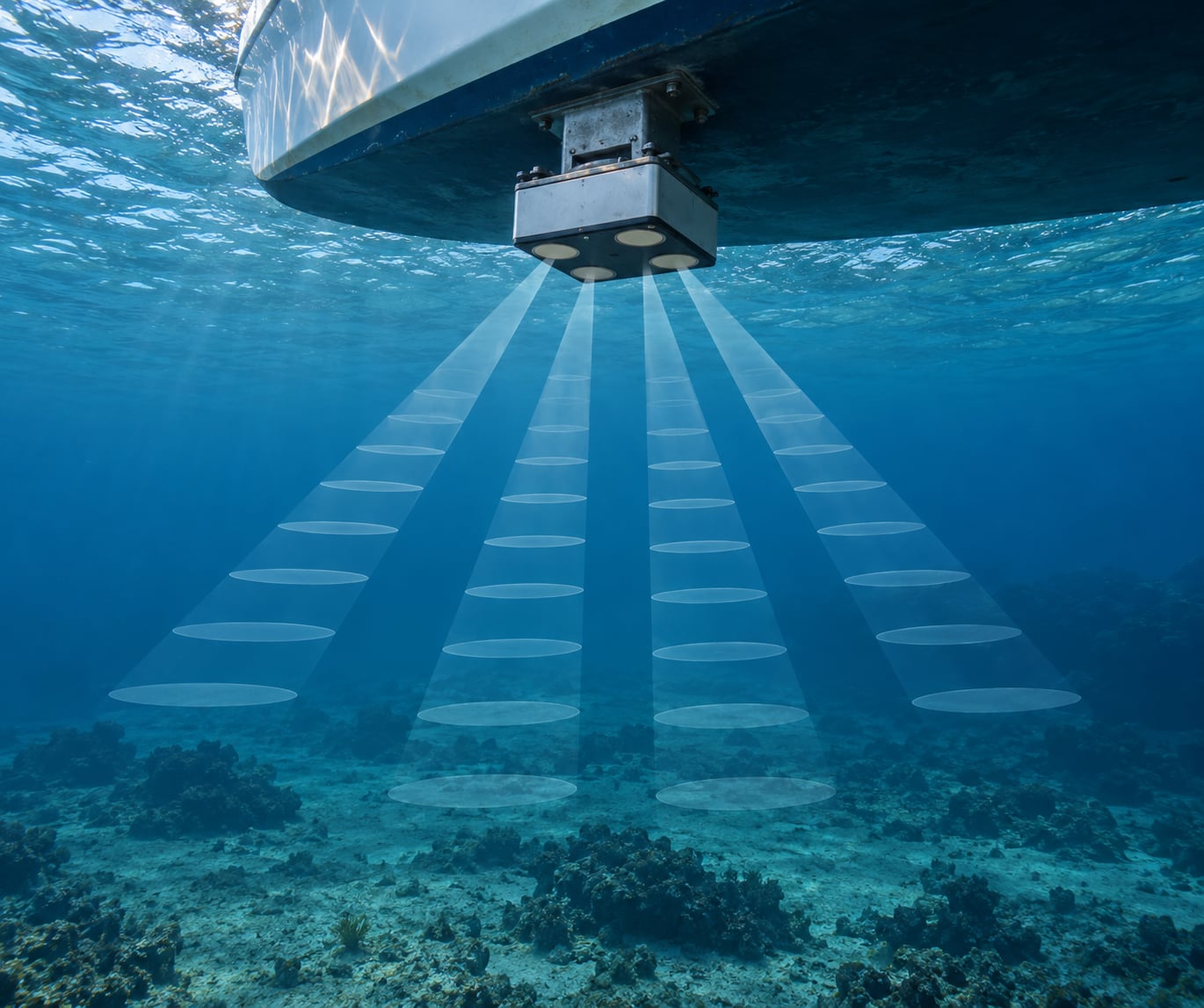
An acoustic Doppler current profiler (ADCP) measures the speed and direction of water currents at every depth through a water column, by listening to the echoes of its own sound pulses bouncing off particles in the water. It records those measurements in layers, so one deployment returns a full vertical profile instead of a single reading.
That is the short version. The detail that trips people up is the line between what the instrument measures directly and what a processing chain computes afterward, because the difference decides whether your data is usable on its own.
Table of Contents
- What an ADCP Measures
- How an ADCP Measures Water Velocity
- What an ADCP Measures at Different Depths
- What an ADCP Does Not Measure
- How ADCP Deployments Are Used in Marine Work
- What Affects ADCP Accuracy and Data Quality
- How to Choose an ADCP for a Deployment
- Frequently Asked Questions
- Start With the Measurement You Need
What an ADCP Measures
An ADCP is a sonar-like hydroacoustic instrument with three or four transducers that send short ultrasonic pulses into the water and listen for the echoes that scatter back. The frequency shift of each echo gives the velocity of the water along that beam.
So what an ADCP measures, directly from the sensor, comes down to a short list:
- Velocity magnitude at each depth cell, split into three components: eastward (u), northward (v) and vertical (w).
- Current direction, derived from the horizontal components relative to the instrument heading.
- Depth of each measurement cell, calculated from the travel time of the echo rather than from a separate sensor.
- Echo intensity, which is a measure of how much acoustic energy comes back from scattering particles in that cell.
- Correlation magnitude and percent good, the two quality flags that tell you whether a velocity estimate is trustworthy.
- Instrument attitude, recorded by tilt, heading and pressure sensors on most models.
- Bottom position, when bottom tracking is enabled and the seabed is within range.
Everything else people call an ADCP measurement is derived. Discharge, or streamflow, comes from the velocity-area method: you multiply each cell’s velocity by its cross-sectional area and sum the columns. A bed profile from bottom tracking is coarse, good enough to know where the bed sits in a river channel but not a bathymetric survey. Turbulence, wave orbital velocity and tidal constituents all come out of post-processing software, not out of the transducers.
One correction worth making early, because it trips up almost everyone new to the instrument. An ADCP does not measure water moving. It measures the motion of the particles suspended in that water, and assumes the water moves with them. In ordinary flows that assumption holds well. In a flow where the water shears past particles that are nearly stationary, the instrument can report a velocity that does not match what a neutrally buoyant float would experience.
How an ADCP Measures Water Velocity
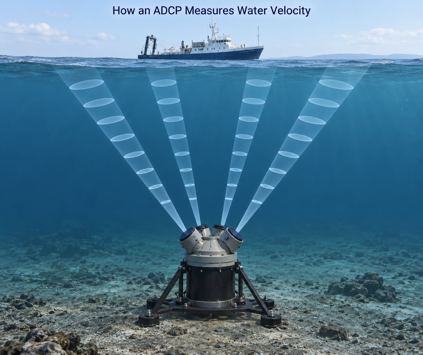
The measurement runs in six steps, repeated as fast as the instrument can ping.
- Transmit. The instrument fires a short pulse of sound along each of its beams at a fixed ultrasonic frequency, typically tens or hundreds of kilohertz. The pulses are microseconds long, which is what gives the instrument its range resolution.
- Scatter. The pulse travels through the water and hits small suspended particles: sediment, plankton, bubbles, debris. Each one reradiates the sound back toward the transducer.
- Listen. The transducer receives the echo a moment later and measures its amplitude and phase relative to the pulse it just sent.
- Apply the Doppler shift. The frequency change between outgoing and returning sound is proportional to the component of particle velocity along the beam axis. Along-beam velocity comes straight out of that.
- Convert range to depth. Travel time to a cell and back gives slant range. Divide by the speed of sound, then correct for the beam slant angle, and you get a distance along the beam and a depth below the face of the instrument.
- Resolve three dimensions. Three beams at known angles give three equations for three velocity components. A fourth beam catches noise in the result and lets the instrument flag it.
Because the instrument knows both how long it took and which beam heard the echo, it can slice the water column into stacked depth cells. Each cell holds one speed, one direction and one set of quality flags, and the cells are usually 10 to 100 cm tall depending on the frequency and the cell size you set.
Most instruments transmit along a slant angle, not straight up. A typical value is around 20 to 30 degrees off vertical. That slant matters for two reasons. It is what lets three beams reconstruct a full three-dimensional vector, and it is also the source of the surface and bottom contamination described later.
How to Read an ADCP Velocity Profile
A velocity profile plot puts depth on one axis and speed on the other, with direction shown as color or as a vector at each cell. Reading one is mostly a process of discarding cells that fail quality checks.
The bottom of the profile usually shows a clear reduction in speed, because friction with the bed slows the near-bed layer. That is real physics, not an instrument error. The same goes for a slower layer under a warm surface on a calm sunny day.
Start at the bottom of the valid record and check the quality flags first. Percent good is the fraction of beams that returned a usable echo in that cell, and it is the flag to trust most. A cell with percent good below roughly 50 percent is usually noise rather than a measurement. Correlation magnitude measures how cleanly the return locks onto the transmitted frequency, and it drops when the signal is weak or the cell contains a mix of moving and stationary particles. Echo intensity falls with range simply because sound attenuates, so a faint cell is not automatically a bad cell.
The first one or two cells below the transducer face are always discarded. The instrument cannot hear inside its own blanking distance, where the near field is full of ringing from the transducer itself.
What an ADCP Measures at Different Depths
How much of the water column an ADCP can cover depends heavily on the setup, and the practical limits come from the geometry rather than the electronics.
| Measurement setup | What it measures well | Practical limits |
|---|---|---|
| Near-surface, side-looking beam | Horizontal currents in the top few metres | Surface return contaminates roughly the outer 10 to 15 percent of the beam path; usable data usually stops well short of the surface |
| Shallow-water, single-cell | One depth of speed and direction | Blank distance leaves the nearest 0.5 to 2 m unusable, which can be most of the water column in a small channel |
| Bottom-mounted, up-looking | Full depth-resolved profile over hundreds of metres | Bottom tracking fails over rough bed; fouling on the transducer face |
| Down-looking from a surface float | Profile from the top of the water column downward | Bubbles and near-surface chop wreck the closest cells; range depends on frequency |
| Vessel-mounted, keel or hull | Continuous profile along a survey track, plus bottom tracking for depth | Needs motion compensation from GPS and attitude sensors; aeration and bubbles from the propeller ruin data |
Lower-frequency instruments reach further because sound attenuates more slowly in water at lower frequencies. A 75 kHz head can profile a deep water column over a kilometre; a 1200 kHz head resolves centimetre-scale turbulence but gives up within tens of metres.
What an ADCP Does Not Measure
Five assumptions show up repeatedly in procurement conversations, and each one costs a team real time.
It is not a depth sounder. The depth of each cell comes from echo timing, but the beam is pointed at the water, not the bed. A bottom-tracking ADCP reports a single bed elevation per ping, which is enough to plot a channel profile and nowhere near enough for a survey.
It is not a CTD. Temperature, conductivity and salinity come from a separate sonde. Many ADCPs log water temperature from a built-in thermometer, and some include a pressure sensor for tide stage, but neither replaces a CTD cast. If you need density or salinity you pair the instruments on the same frame.
It is not a turbidity or sediment sensor. Echo intensity responds to how much material scatters sound, so a backscatter profile correlates with suspended sediment in a given site. Turning that into a sediment concentration requires a local calibration curve, and the calibration is site-specific. Anyone quoting a concentration straight from raw echo intensity without a rating curve is guessing.
It does not resolve horizontal velocity well from a side-looking beam. A beam aimed horizontally along the flow has a very small radial component of the velocity it is trying to measure, so the Doppler signal is weak and the uncertainty is large. Instruments that need reliable horizontal flow at one depth use a down-looking cell or a tilt trick with an array instead.
It does not measure the water itself. Back to the scatterers. In highly stratified flows or around bubble plumes, the particles and the water can genuinely disagree.
How ADCP Deployments Are Used in Marine Work
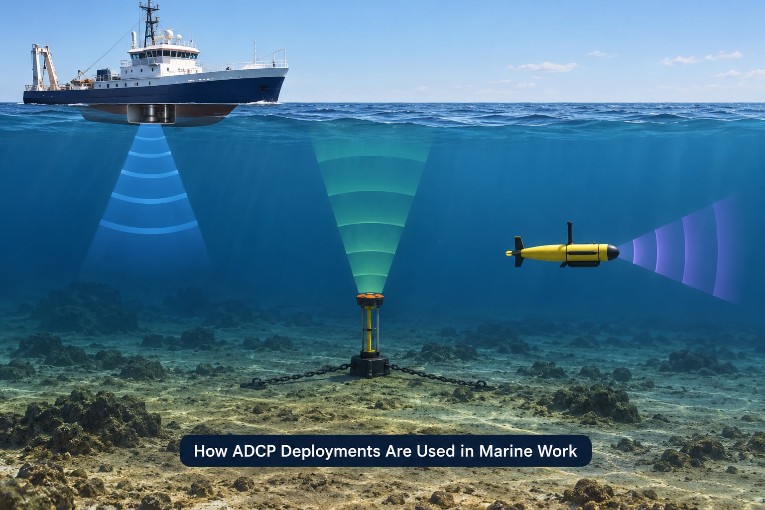
Where you put the instrument decides which questions it can answer.
Hull-mounted on a survey vessel is the standard hydrographic setup. Combined with GPS and an attitude reference it produces a continuous profile along the track, and bottom tracking gives water depth at the same time, which removes the need for a separate echosounder on short surveys. The hard part is avoiding aerated water. Propeller wash and hull bubbles scatter sound so strongly that the nearest cells are unusable during acceleration or in a following sea.
Bottom-mounted upward-looking deployments sit on a seabed frame or a pier leg for weeks or months, logging the tidal cycle and any storm signal. This is where you get long time series rather than snapshots. It is also where biofouling matters most, because a barnacle layer on the transducer face attenuates the outgoing pulse and the return together.
Side-looking or vertical mounts on bridge piers, pilings and quay walls measure the near-surface current in a harbour approach or a shipping channel without putting a boat in the way.
Moored upward-looking on a buoy combined with a downward-looking unit on the mooring line gives a profile that spans both the surface layer and the deeper column in one mooring.
Lowered through the water column from a small boat gives a full-depth cast without a mooring, which is how most of the deep ocean work is done.
On a moving underwater vehicle, an ADCP becomes a Doppler velocity log. A vehicle-mounted downward-looking unit locks onto the seabed and measures the vehicle’s speed over ground by subtracting the water velocity from its own motion. This is the link that puts ADCP technology directly into ocean robotics: the same instrument that a hydrologist leaves on a riverbed for a season is, in a different housing, the navigation reference an AUV uses to know where it is.
Along the way, the derived quantities earn their keep. Combining the velocity profile with tide stage and channel geometry gives discharge. Removing the depth-mean flow leaves the residual and the variance, which describes turbulence. Isolating the periodic component at wave frequencies leaves wave orbital velocity.
What Affects ADCP Accuracy and Data Quality
Most disappointing ADCP datasets come down to one of a handful of physical problems, and they are worth recognising in the data.
Not enough scatterers. An ADCP needs suspended particles. In very clear water, the echo weakens with range until the correlation drops and the cells go bad. Coastal and estuarine water is usually forgiving; clear offshore or polar water is not.
Bubbles. A breaking wave, a bubble plume or propeller aeration produces a wall of strong scatterers, and the instrument reports a velocity that reflects the bubble motion rather than the flow. Cells with sudden, isolated speed spikes and unusual echo intensity are usually this.
Sidelobe interference. A transducer beam is not a laser. Energy leaks sideways at lower levels, and that energy hits the surface or the bed and returns to confuse the measurement. The effect reaches roughly 86 percent of the distance to the surface at a 30 degree slant angle, which is why the top cell in a vertical beam is almost always discarded.
Boundary layers. Near-bed cells are physically different because of friction, and near-surface cells are disturbed by wind and waves. Do not treat those gradients as instrument error, and do not average across them.
Strong vertical motion. Waves that move the water faster than the depth cell is tall mix the water inside a cell, which smears the profile. Fine cells at higher frequency help, and wave averaging software handles the rest.
Tilt and heading. Beam angles are calculated in instrument coordinates. If the instrument tilts and the tilt sensor is missing or wrong, the vertical velocity comes out wrong. A vessel-mounted unit with a bad compass gives a right speed and a wrong direction, which is a confusing failure to diagnose in the field.
Electrical noise and timing. Motor controllers, acoustic releasers and bad grounding show up as correlation collapse and phantom velocities in specific cells. A magnetometer near current-carrying mooring hardware gets the same treatment.
Motion in the mooring. A frame swinging in a current changes the depth assigned to each cell. Pressure and tilt sensors correct for it, and without them the profile smears over a tidal cycle.
How to Choose an ADCP for a Deployment
Work through these in order, because each one narrows the choice more than the last.
Define the depth range first. The range you need sets the frequency. Shallow and turbulent work wants a high-frequency head measured in centimetres to decimetres of cell size; deep coastal and ocean work wants a low-frequency head with cells in metres.
Then set the mounting method. Hull-mounted, bottom-mounted, moored, lowered and vehicle-mounted units have different form factors and power budgets. A unit that needs a survey vessel is the wrong tool for a bridge pier, and a shallow draft unit may not be able to profile the depth you care about.
Match the velocity you expect. Check the instrument’s velocity range against your site. A unit with a 0.3 m per second ceiling in a tidal channel with a 2 m per second peak will return clipped, aliased values that look like real flow if you do not check the flags.
Plan power and telemetry. Ping rate is the largest single drain on the battery. Every ping is a full transmit and a full listen, so doubling the ping rate halves the deployment length. Work out the duty cycle from your sampling requirement, then size the battery against it rather than against the best case.
Decide whether you need real-time data. Self-logging units record everything and cost less in telemetry. If the measurement has to trigger a response, you need a radio or satellite link, and that changes the power budget substantially.
Match the pressure rating to the deepest deployment. A unit rated for shallow water will fail at depth, and it will fail silently at first as the housing takes on water.
Be honest about the secondary variables. If the project also needs salinity, turbidity or sediment concentration, budget for a CTD, an optical backscatter sensor and the calibration work that goes with them. Pairing them on one frame is cheaper than deploying separately.
What an ADCP Measures at Each Frequency
| Frequency | Typical profiling range | Typical cell size | Typical use |
|---|---|---|---|
| ~75 kHz | Several hundred metres to over 1 km | Metres | Oceanographic moorings, deep water profiling |
| ~150 to 600 kHz | Tens to hundreds of metres | Decimetres to half-metre | Coastal, harbour, estuarine and vessel surveys |
| ~600 to 1200 kHz | Tens of metres | Centimetres to decimetres | Turbulence, waves, laboratory flumes, shallow channels |
| 1 to 10 MHz | Under 10 metres | Centimetres | Laboratory flumes, very shallow water |
These are representative ranges rather than specifications. The same frequency behaves differently depending on cell size, processing mode and how much scatterer material is in the water.
Frequently Asked Questions
Does an ADCP measure depth or water depth?
It measures the depth of each of its own data cells, derived from echo travel time, not the depth of the water. Total water depth is a separate quantity: it comes from a pressure sensor or from bottom tracking when the instrument can lock onto the bed. That bottom-tracking depth is a single elevation per ping, useful for plotting a channel profile but not a substitute for a bathymetric survey.
What is the difference between an ADCP and a CTD?
They measure different things entirely. An acoustic Doppler current profiler measures water velocity through a depth range using the Doppler shift of reflected sound. A CTD measures conductivity, temperature and depth to derive salinity and density. In practice the two are mounted together on the same frame, because a current profile without density context tells you very little about how that water moves.
Can an ADCP measure vertical water velocity?
Yes, and that component is called w. It comes from the combination of the slant beams rather than from any single beam aimed straight up, which is why at least three beams at known angles are needed. Vertical velocity is usually small, so it is also the component most easily corrupted by tilt error, wave motion and boundary layer contamination near the surface and the bed.
What does bottom tracking mean on an ADCP?
Bottom tracking is a processing mode where the instrument looks for a strong return from the seabed and treats it as a reference layer. Two things follow from that: it records the bed depth at that horizontal position, and it gives a speed over ground that is independent of the water velocity. That speed is what a vehicle-mounted unit uses to navigate. Over a rough or mobile bed the return is unreliable, and the flag for it is the bottom-track quality indicator.
How often should an ADCP be calibrated?
Before every deployment, and more often than people expect. Check the transducers for fouling and clean them, verify the clock against GPS, confirm the sound speed setting against a contemporaneous cast, and check the compass calibration on a vessel-mounted unit. Long moored deployments need a mid-deployment recovery for inspection. Calibration drifts mostly from fouling, magnetometer interference and clock error rather than from the electronics themselves.
How accurate are ADCP measurements?
In good conditions a well-configured instrument holds velocity to roughly the better of 1 percent of measured speed or 0.5 cm per second, which is why the accuracy is quoted as a fraction of the reading rather than a fixed number. In practice the error is usually set by the environment: weak scatterers, bubbles, sidelobe contamination at the surface and seabed, and tilt errors on moving mounts all push uncertainty above the instrument specification.
Start With the Measurement You Need
Write down the depth range, the velocity accuracy, the deployment geometry and the supporting variables before you look at any instrument. That short list usually decides the frequency class, the mounting method and the power budget before you compare anything.
Then remember the split. Velocity components and cell depth come straight from the sensor. Discharge, bed profile, turbulence and wave orbital velocity are derived, and they depend on settings, quality flags and processing software. If your project needs the derived numbers, budget for post-processing as well as for the instrument.
Once that dataset exists, the open route is well trodden: USGS technical manual 3-A22 covers discharge measurement in depth, and CODAS is the standard open processing chain most practitioners reach for. Getting from a raw binary file to a trustworthy profile is the part that catches newcomers out, and it is worth planning for before the instrument goes in the water.