Microplastics are collected by taking a known volume of water or a known mass of sediment, capturing every plastic particle above a stated size threshold on a filter, and keeping that volume or mass free of plastic added from your own gear. Counting is the separate step: sorting, sizing and tallying the captured particles under a stereomicroscope, then confirming polymer identity with a spectroscopic method. Both halves have to be documented, because a count without a size threshold and a blank correction is not a measurement.
This guide walks the whole route from the water surface to a reportable number, because that is how microplastics are collected and counted in practice. It is written for people who have to make the calls themselves: coastal monitoring groups, university researchers, drinking water and wastewater teams, and classroom or volunteer projects working with basic equipment.
Table of Contents
- What Does Collecting and Counting Microplastics Involve?
- How Microplastics Are Collected from Water
- How Samples Are Prepared Without Adding Plastic Fibers
- How Microplastics Are Identified and Classified
- How Microplastics Are Counted and Reported
- How Microplastics Are Collected and Counted in Sediment and Biota
- What Quality Controls Make the Results Trustworthy?
- Frequently Asked Questions
- What is the smallest microplastic that can be reliably collected?
- Is a larger water sample always better for microplastic analysis?
- How do laboratories confirm that a particle is plastic?
- How much microplastic contamination comes from sampling equipment and handling?
- Should suspected particles be counted individually or by weight?
- What units should a study report for microplastic abundance?
- Start with a Method That Matches the Question
What Does Collecting and Counting Microplastics Involve?
A microplastic is a synthetic polymer particle smaller than 5 mm. Below that, working scientists usually work in narrower bands, because a 300 µm count and a 20 µm count are entirely different measurements of the same water.
Most working definitions set the lower limit at 1 mm, with 300 µm common for marine surface work and 20 to 25 µm treated as the practical floor for routine optical identification. Below roughly 20 µm, a particle is smaller than many counting grid cells and identification stops being a visual exercise. Size alone is not enough, though. A fibre off a fleece jacket, a paint chip, a glass fragment and a cellulose fibre all look similar at 80x magnification, which is why confirmation comes later in the pipeline.
The work runs in seven stages, and each one is a place to lose particles or invent them:
- Define the measurement — count, size distribution, polymer identity or mass, plus the size threshold.
- Collect — a known volume of water or a known dry mass of sediment, using gear with no plastic parts in the flow path.
- Blank — run field and procedural blanks so the plastic coming from your own equipment is measurable and subtractable.
- Digest — break down organic matter so plastic can be seen and separated.
- Separate and filter — isolate plastic by density, then capture it on a pre-weighed membrane.
- Count and size — systematic microscope sweep, morphological classification, size binning.
- Confirm and report — polymer identification on a representative subsample, then report with threshold, blanks and units attached.
| Stage | What it produces | Where it usually fails |
|---|---|---|
| Definition | Size threshold and target measurement | No threshold stated, so results cannot be compared |
| Collection | Water volume or sediment dry mass | Unknown volume, or plastic tubing shedding fibres |
| Blanking | Contamination estimate per stage | Skipped, or blanks handled in the lab instead of the field |
| Digestion | Particle-free matrix | Aggressive chemistry embeds or breaks up small particles |
| Density separation | Plastic-rich fraction | Solution density too low for the target polymer, or toxic |
| Filtration | Particles on a membrane | Membrane clogs, particles pass through mesh edges |
| Counting | Abundance and size distribution | Double counts, missed edge particles, ambiguous picks |
| Confirmation | Polymer identity | Visual-only identification reported as certain |
How Microplastics Are Collected from Water
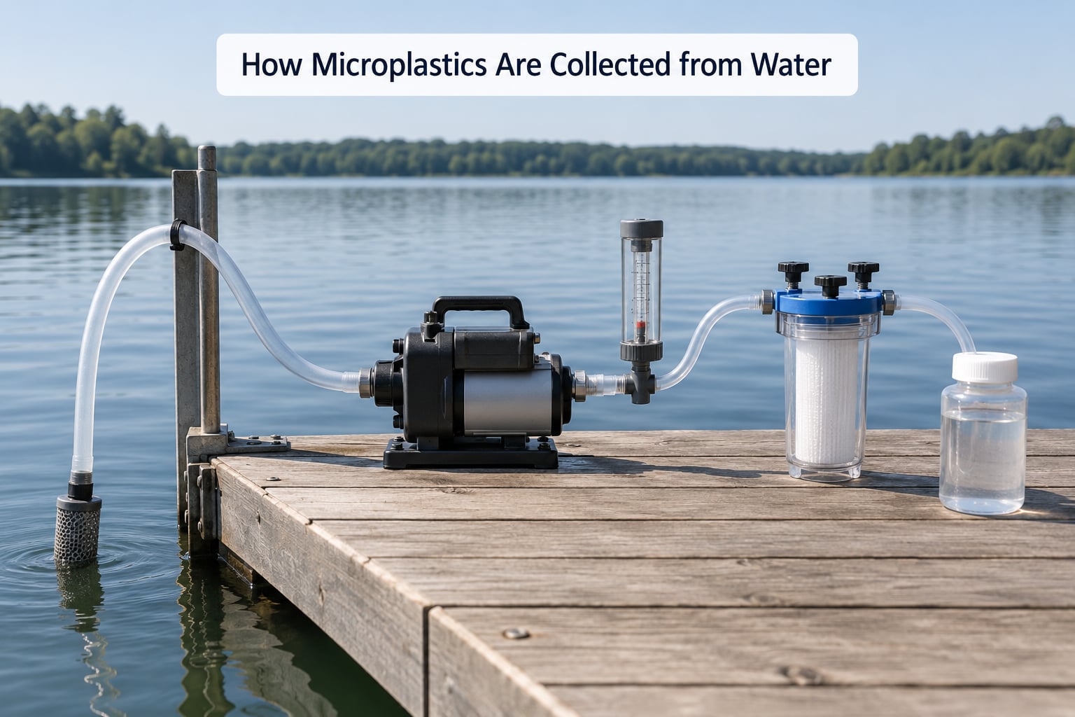
Water sampling comes in three families, and the choice is driven entirely by the volume you need and the particle size you intend to catch. Anything below 300 µm requires a different gear set from anything above it, no matter how clean the method looks on paper.
| Method | Typical volume | Size captured | Best for |
|---|---|---|---|
| Bulk grab | 1 to 20 L | Above roughly 300 µm | Harbours, estuaries, small studies, classroom work |
| Pump and stack | 20 to several hundred L | Above 10 to 50 µm with a finer stack | Coastal programmes, wastewater and influent work |
| Manta trawl | Over 1000 L per haul | Above 300 µm typically | Open-ocean surface surveys and transects |
| Glass funnel and filter | 0.5 to 2 L | Down to about 20 µm | Drinking water, volunteer sampling, small volumes |
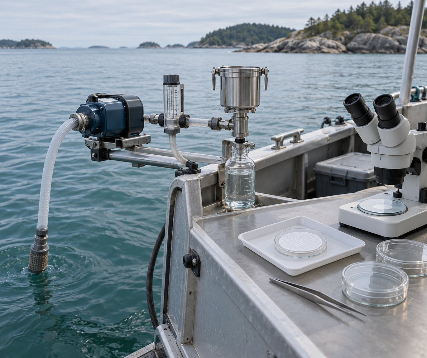
For a pump system, the sequence at the start matters more than people expect. Prime and flush the line with sample water, discard the flush volume, then start collecting and record the flow meter reading at the beginning and end of each sample. In practice the volume is the back-calculation from those two readings, multiplied by the time elapsed, and it is the number that later turns a count into particles per litre.
Depth is a design decision, not a detail. A surface skim samples a different particle population than a depth-integrated bottle cast or a mid-water intake, so mixing the two into one number describes nothing. Coastal programmes commonly pair a surface skim with a shallow profile cast so the vertical difference is visible rather than averaged away.
Between samples, everything gets rinsed with pre-filtered water, and the rinse goes into the field blank bottle rather than down the drain. Weather, wind, swell state, tide, depth, time of day and exact coordinates belong on the label, because these are the variables that make a count reproducible six months later. A label that only carries a site name is a number nobody can repeat.
How Samples Are Prepared Without Adding Plastic Fibers
Contamination control is the part that decides whether your number means anything. The biggest source of error is not the sample; it is the sampler’s own clothing, gloves, bottles, tubing and lids shedding fibres into the bottle while you are trying to measure somebody else’s particles. That is the single most repeated complaint in volunteer and student microplastic work, and it is why working protocols start with what you are wearing, not with the water.
Wear cotton or other natural-fibre clothing rather than fleece or polyester, and avoid synthetic gloves, synthetic hair ties and waterproof shells. Use glass or 316 stainless steel for anything that touches the sample, and keep consumables such as membranes and filters in sealed glass or foil packaging rather than plastic bags. A cotton lab coat is the single most effective swap anyone can make.
Once in the lab, the aim of preparation is to leave a matrix with no organic matter and no mineral grit, so the remaining particles are almost certainly plastic.
Digestion removes biological and organic material. The method depends on what you are holding, not on preference: a wet, organic-rich sediment or gut content responds to a different chemistry than a seawater filter, and a shell or faecal pellet needs something stronger than a seawater filter will tolerate.
| Matrix | Digestion approach | Watch for |
|---|---|---|
| Seawater filter | Enzymatic or mild oxidative digestion | Over-oxidation crazes weathered plastics, raising the count |
| Organic-rich sediment | Stronger oxidative digestion with heating | Airborne fibres during long heating steps |
| Biota tissue | Enzymatic or oxidative digestion of tissue | Loss of small fragments; unremoved gut contents bias the count |
| Sandy or mineral sediment | Digestion plus density separation | Mineral carry-over that obscures particles on the membrane |
Density separation works because most common polymers float in a solution denser than water. Plastic is trapped at the surface, denser mineral grains sink. The choice of solution sets your recovery and your hazards.
| Solution | Typical density | Character |
|---|---|---|
| Potassium iodide | About 1.6 g/cm3 | Low cost, recoverable, but corrosive and stains particles |
| Zinc chloride | About 1.6 to 1.7 g/cm3 | Good recovery, cheap, but acutely toxic to handlers |
| Sodium iodide | About 1.8 g/cm3 | High recovery across polymer types, expensive, requires heating |
| Zirconium chloride | About 1.6 to 1.8 g/cm3 | Very high recovery, aggressive, needs strict handling control |
Whatever you use, the method needs a recovery test: spike a known number of plastic reference particles into a blank matrix and see how many come back. Recovery is usually quoted as a percentage, and a method that recovers a fraction of what you put in quietly under-reports the environment, not the sample.
Two blank types do the contamination accounting. A field blank is a bottle of fully filtered water carried through the entire sampling procedure on the boat, so it captures contamination from the boat, the deck, the handling and the bottles. A procedural blank is taken through the whole lab protocol in the cleanest possible conditions. Comparing them tells you whether the contamination arrived in the field or in the lab, and that difference changes what you fix.
How Microplastics Are Identified and Classified
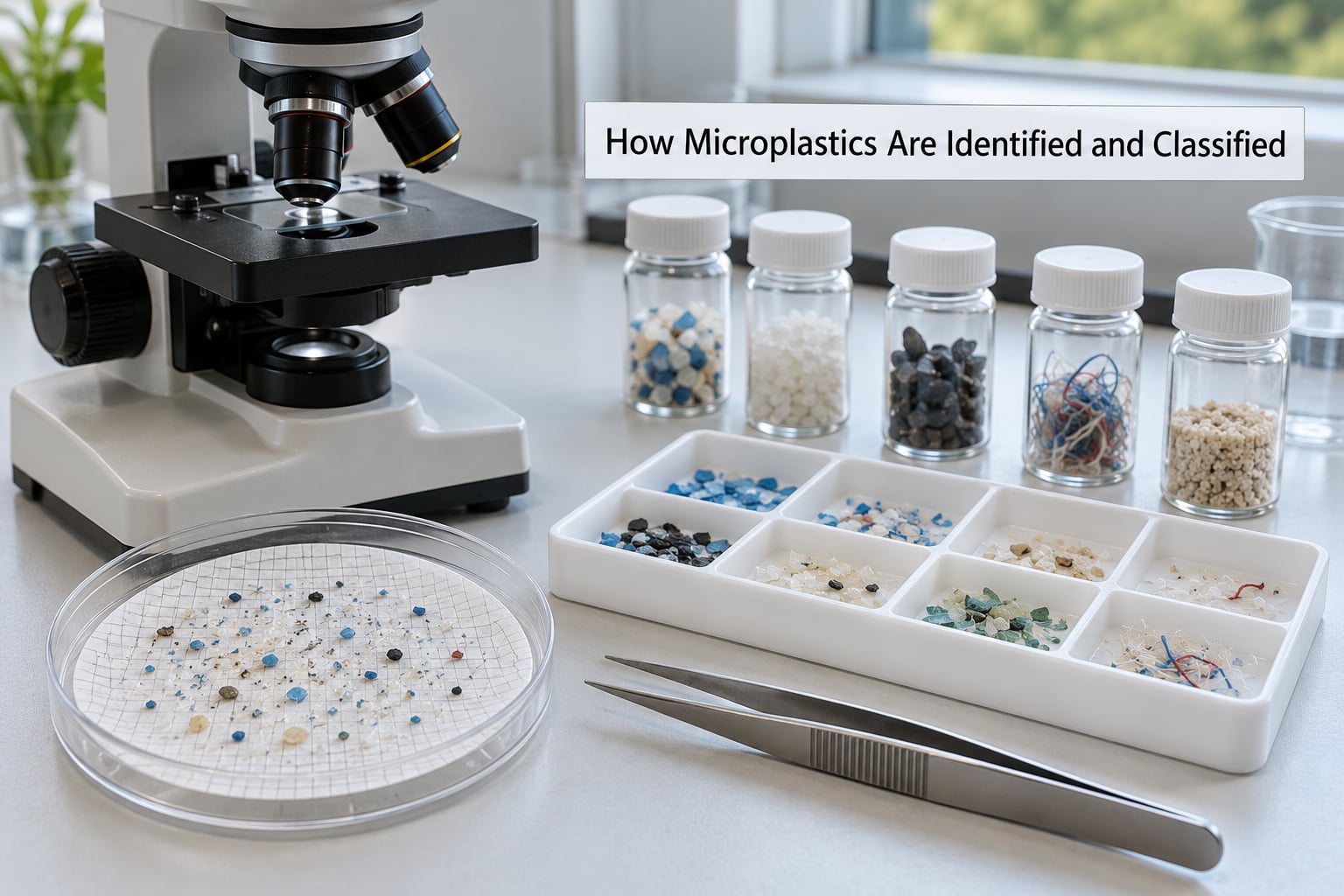
Identification splits into two jobs that people often blur together. Classification is the human judgement call: is this a fibre, a fragment, a film, a foam bead, a paint chip or a non-plastic inclusion, and what colour is it. Confirmation is the instrument answering what the polymer is. A visual count is a count of candidate particles, not of confirmed plastic, and saying so is the difference between a screening result and a study result.
Shape classes follow a standard vocabulary — fibre, fragment, film, foam, bead, and sometimes paint chip and rubber. Colour is graded against a fixed chart, not described as “blue-ish”, because a reproducible report needs a category another analyst would also have chosen.
Visual screening typically rules out obvious non-plastics: mineral grains, cellulose and cotton fibres, glass shards, insect parts, and the regular textile weave of clothing fibres seen down a microscope. It cannot resolve clear plastic from clear plastic of a different resin, and that limitation is exactly what spectroscopy was built to fix.
| Method | What it tells you | Minimum size | Destructive | Throughput |
|---|---|---|---|---|
| Stereomicroscope | Count, size, shape, colour | About 20 µm | No | High, but analyst-dependent |
| Staining such as Nile Red | Pre-screen, highlights organic residue | About 20 µm | No | High; risks false positives |
| FTIR | Polymer identity from infrared absorption | About 10 to 20 µm in transmission, 500 µm mapped on some systems | No in reflection modes | Medium to high |
| Raman | Polymer identity, works through containers | About 1 µm | No | Low to medium; fluorescence interference from pigments |
| O-PTIR | Polymer identity combined with spatial mapping on a single particle | About 500 nm | No | Low, research grade |
| Py-GC-MS | Mass concentration by polymer, no particle count | Not particle-resolved | Yes, the whole sample is consumed | Low, but very specific |
Two practical notes from real workflows. Raman is vulnerable to fluorescence from pigments and leftover organic matter, which is why a blank matrix matters as much for spectra as for counts. And a review of detection methods published in 2026 made the same point this guide is making from the other end: there is no single method that answers every question, so equipment gets chosen by measurement requirement, not by reputation.
Automated and machine-vision counting sits in the middle of this table rather than replacing it. It speeds up tallying and size measurement on a loaded filter and reduces the fatigue that causes missed and double counts, but it does not change the chemistry, and it still needs a human check on a subset. A recent review makes that same distinction: AI changes the workflow, not the underlying method.
How Microplastics Are Counted and Reported
Counting by hand follows a fixed procedure so results do not depend on who was at the microscope. The method that works at any size is a systematic sweep, in which you divide the membrane or petri dish into fields, work across in one direction without skipping, and count only what falls inside the field, which removes edge double-counting as a decision.
The routine runs like this:
- Clean the work area, lay out covered glass dishes, and open only one sample at a time.
- Place the membrane on a gridded background and start at a fixed reference point, usually a marked corner or a membrane edge notch.
- Work in bands across the filter, field by field, counting within defined field boundaries only.
- For every candidate particle, record the size in its longest dimension, the shape class and the colour grade.
- Move each counted particle into a covered dish or a marked map so the same particle is not tallied twice.
- For dense filters, count a defined fraction or a set number of fields and extrapolate, then say so in the report.
- Re-read a random subset of fields to estimate analyst counting error before finalising the total.
Small-particulate protocols often add grid counting with gridded eyepieces, which reduces the number of fields needed. Whatever the variant, the counting rules must be written down before counting starts, not after the numbers look wrong.
Counting and identification are then reported separately. A typical result states a particle count in the fraction above a named threshold, a size distribution in stated bins, a polymer breakdown from a representative subsample, and the blank correction applied to each.
| Unit | What it means | Typical use |
|---|---|---|
| Particles per litre | Count divided by filtered water volume | Surface water, drinking water, wastewater |
| Particles per cubic metre | Same, scaled for large water bodies | Ocean and estuary transects |
| Particles per kilogram dry weight | Count divided by dry sediment or tissue mass | Beach and seabed sediment, biota |
| Mass in milligrams per kilogram | Polymer mass rather than particle number | Py-GC-MS style results, sediment |
Two numbers from the same water are not comparable until you know whether one counts above 1 mm and the other above 25 µm, and whether one is blank-corrected. That single fact explains most of the wild spread in published figures, and it is not evidence that the ocean changed.
How Microplastics Are Collected and Counted in Sediment and Biota
Sediment and tissue need their own methods because both are dominated by mineral or organic mass that the water method never sees. In both cases the count is normalised to dry weight, so drying and pre-weighing the matrix is not optional bookkeeping, it is part of the measurement.
| Matrix | Collection | Key processing step | Reported as |
|---|---|---|---|
| Beach and seabed sediment | Shallow corer or quadrat, transect-based | Dry sieve, digest, density separate | Particles per kg dry weight |
| Sediment traps | Time-series trap, usually at a fixed mooring | Wet sieving then the water workflow | Particles per square metre per time period |
| Benthos and shellfish | Grab or dredge, whole soft tissue | Digest tissue, inspect gut contents separately | Particles per individual or per kg wet weight |
| Fish gut contents | Whole organism or dissected gut | Enzymatic digestion of gut material | Particles per organism |
For sediment, the practical classroom method is small and legible: dry a weighed aliquot, put about 3 g into a glass petri dish, and sweep the dish systematically under a stereomicroscope, exactly the way you would count the water filter. Larger programmes sieve first, then run the retained fraction through the full digestion and density separation workflow, and report recovery for the spikes they added.
For biota, the standard is to digest the soft tissue only, keep shell material out of the sample, and decide in advance whether gut contents are included. Unremoved gut material inflates counts with non-plastic inclusions, and an unfiltered gut read is a frequent source of disagreement between laboratories working on the same species.
What Quality Controls Make the Results Trustworthy?
Trustworthy microplastic data comes from controls that are run every time, not from a more expensive instrument. The list below is short enough to actually follow, and every line maps to a documented practice in institutional sampling guidance.
- Field and procedural blanks on every trip and every batch, reported alongside the samples they correct.
- Recovery tests with known reference particles at more than one size, since recovery falls as particles get smaller.
- A stated detection limit and size threshold in every result, including the fraction below which particles were not counted.
- Chain-of-custody records covering who handled the sample, when, and under what conditions.
- Analyst consistency checks by re-reading fields, plus interlaboratory comparison when your data will be compared with published work.
- Full metadata with every count: mesh size, filtered volume or dry mass, digestion chemistry, separation solution and its density, membrane type, counting rules.
- Uncertain or ambiguous particles reported as uncertain, kept as a separate category rather than quietly counted or discarded.
Also worth stating plainly: there is no broadly agreed global standard for this workflow yet, which is why protocols in the wild range from a university classroom handout to multi-agency operating procedures such as the Southern California Coastal Water Research Project’s trash and microplastics SOP, and why USGS, EPA and regional monitoring programmes publish guidance rather than a single fixed method. Standardisation, not detection hardware, is the open problem in this field.
Drinking water work uses the same logic with a different front end, where a small volume is filtered and a large one is sampled, which is why drinking water results concentrate in the small-particle fraction. Brand-to-brand comparisons drawn from different studies do not hold up, because the thresholds and methods behind them differ.
Frequently Asked Questions
What is the smallest microplastic that can be reliably collected?
For routine optical work, 20 to 25 µm is the practical lower limit: below that, particles are too small to classify reliably under a stereomicroscope and are easily missed. Routine marine monitoring often sets a higher floor, commonly 300 µm, because that is what a trawl mesh captures. Finer collection is possible with stacked filtration and confirmed by Raman or O-PTIR, but it costs time and recovery drops as size falls. Always report the threshold used.
Is a larger water sample always better for microplastic analysis?
No. A bigger sample reduces the limit of detection and gives more particles to classify, but it also means more contamination, more clogging and more handling. Beyond a few hundred litres, the returns flatten while the blank burden keeps growing. Many programmes settle on 20 to 100 L per replicate because the extra statistical value no longer pays for the added contamination risk.
How do laboratories confirm that a particle is plastic?
They measure a spectrum and match it against a reference library of polymer fingerprints. FTIR compares infrared absorption to known resins, Raman compares shifted laser wavelengths and reaches far smaller particles, and O-PTIR maps chemical composition across one particle. Py-GC-MS takes a different route, burning the sample to measure polymer mass, which gives a concentration but no particle count and no size information.
How much microplastic contamination comes from sampling equipment and handling?
Often enough to invert a result. Fleece jackets, synthetic gloves, sample bottles, tubing, zip ties and even the lid seal can each shed fibres, and those fibres are indistinguishable from the sample by eye. That is why field blanks are opened alongside samples, and why cotton clothing, glass or stainless steel hardware, and glass or foil packaging for consumables are standard practice rather than optional care.
Should suspected particles be counted individually or by weight?
They answer different questions, so serious studies report both when they can. Individual counting gives abundance, size distribution and shape class, which is what ecology and most monitoring programmes need. Mass measurement via thermal analysis gives polymer concentration but no count and no particle numbers. A count alone is a screen; a count with a polymer confirmation on a subsample is a defensible result.
What units should a study report for microplastic abundance?
Use particles per litre for water, particles per cubic metre for ocean and estuary transects, and particles per kilogram dry weight for sediment and biota. Attach the size threshold, the filtered volume or dry mass, the mesh size and the blank correction to every figure. Without those four details, the number cannot be compared with another study, which is the most common reason published figures appear to disagree.
Start with a Method That Matches the Question
Before choosing a filter, a net or a separation solution, write down four things: the matrix (water, sediment or tissue), the size range you care about, the sampling location and depth, and the comparison you intend to make. Those four lines decide the gear, the chemistry and the units, and they take ten minutes.
That is how microplastics are collected and counted into something a second team can repeat: a stated threshold, a known volume or dry mass, a blank for every stage, particles tallied on a fixed sweep, and polymer identity confirmed rather than assumed. Start with a small pilot and a few blanks, get the contamination under control, and only then scale up.