Anyone asking how to measure underwater noise ends up doing the same three things: drop a hydrophone into the water, record the signal it produces as an electrical voltage, and convert those volts into decibels referenced to 1 micropascal. The hard part is not the dropping, it is everything around it: choosing a sensor with a low enough self-noise floor, deploying it so the water moving over it does not swamp the recording, and calibrating it so your numbers mean something to anyone who reads them. A first sensible deployment takes an afternoon and a short boat trip. A defensible environmental noise baseline takes weeks of planning before the boat ever leaves the dock.
This guide walks the whole chain, from deciding what you are trying to find out to writing up the result. It is written for people who need real numbers, whether you are a marine consultant, a student building a first recorder, or a maker who wants their data to hold up outside their own notebook.
Table of Contents
What You Need
The full chain runs sensor to preamplifier to digitiser to storage. Every stage adds noise of its own, and the weakest stage sets your floor.
- A hydrophone. A transducer that converts acoustic pressure in water into voltage. Most are piezoelectric ceramic; some are fibre-optic or MEMS-based, which matters mainly when you need high dynamic range or immunity to electrical interference.
- A low-noise preamplifier. Not an audio preamp with a gain knob. A low-noise instrumentation amplifier sets the noise floor you will actually hit at quiet sites.
- Data acquisition. A dedicated recorder or audio interface with a sample rate you can set. A sound card can work for a first pass but rarely gives you a documented noise floor.
- A computer and analysis software. Anything that shows a waveform and a spectrogram will do. Dedicated tools such as PAMGuard, Raven or SoundScope add detection, annotation and batch processing.
- Calibration reference. A pistonphone, a known reference transducer, or a signal generator traceable to a standard. Without one you can compare runs against each other, but you cannot claim absolute levels.
- Site information. Charts, depth, distance to the source, expected traffic, tidal state and a note of what else was happening in the water. Half the mystery in a noisy recording is a second source you did not know about.
- Mooring hardware and safety kit. Floats, ballast, line, shackles, a depth sounder, a hand line, a knife, a spare battery, and a personal flotation device for everyone on deck.
Two consumables catch people out. Bring spare storage or work out the arithmetic before you leave: at 96 kHz and 24-bit you generate roughly 2.8 MB per channel per minute, which is about 4 GB an hour on a single channel. A week-long continuous deployment on four channels is around 700 GB, so a duty cycle or a smaller file format changes what is possible.
Step-by-Step
1. Define the Goal Before You Measure Underwater Noise
Write the objective down as a sentence with a number in it. “Characterise ambient noise” is not an objective. “Establish a baseline at 20 m depth in the outer channel, 10 Hz to 20 kHz, over a full spring tide cycle so the pile driving and the tide can be separated” is.
Six things need pinning down before you pick equipment:
- The source. Ambient, a specific vessel, pile driving, a tidal turbine, a reef, or your own robot. Ambient work and event work need different instruments and different record lengths.
- The frequency band. Most ocean noise energy sits below a few hundred hertz; shipping tones and small pumps can reach tens of kilohertz. Recording wider than you need costs storage and pulls in more self noise.
- The duration. A single pass tells you little. Tides, weather and traffic all cycle on periods of hours and days, and a compliant baseline usually needs a full tidal cycle at minimum.
- The location and depth. Depth changes what you hear, because surface wind and wave noise fall off with depth while distant low-frequency sources arrive almost unchanged.
- The comparison condition. The “before” measurement. If you are assessing an impact, the baseline has to sit in the same place, season and state as the later measurement or the comparison is worthless.
- The output. Broadband level, octave band levels, spectrograms, a detection count, an exposure model. The output decides the sampling rate and the processing.
Getting this written down takes twenty minutes and saves the deployment. On a bioacoustics Stack Exchange thread, people keep circling back to the same realisation: most disappointing recordings are not bad instruments, they are unanswered questions recorded for too short a time.
2. Select the Right Hydrophone
A hydrophone is chosen by four numbers, and only four: the frequency band you need, the self-noise floor below that band, the sensitivity in your signal chain, and the dynamic range between the two.
Passive versus active. A passive hydrophone only listens. An active one also transmits, which is what you need if you are pinging a target or doing sonar work, and which adds electronics noise you would rather not carry into a quiet measurement.
Self noise is the electrical noise the instrument makes on its own. It is quoted as an equivalent input noise level across the band, and it is the number that decides whether a quiet site is measurable at all. Sensitivity tells you how many volts you get per micropascal; a more sensitive sensor needs less preamplifier gain, and less gain means less added electronic noise.
Frequency response is rarely flat. A flat-response instrument is expensive but predictable. A shaped one, common in marine mammal work, boosts a band where the target lives at the cost of usable range elsewhere. Dynamic range is the gap between the faintest and loudest thing it can record before clipping, and pile driving is where this matters.
How far a hydrophone can hear is set by spreading and absorption rather than by range alone. Low frequencies travel for tens of kilometres in seawater; a few kilohertz is absorbed within a few hundred metres. In freshwater the picture changes again, with much shorter ranges and more influence from the riverbed and banks.
Here is how the practical tiers line up. What each one can support matters more than what it costs.
| Tier | What it can support | Calibration | Main limitation |
|---|---|---|---|
| DIY capsule build (electret capsule in an oil-filled housing) | Relative comparisons, spotting events, teaching, bioacoustic survey at a screening level | None, or a single point gain from a reference signal | Unknown sensitivity, wide tolerance between builds, no frequency response data, hydrostatic pressure changes the response |
| Calibrated mid-tier hydrophone with a data logger | Quantified ambient levels, octave band reporting, construction monitoring with a defined uncertainty | Pistonphone before and after deployment | Still not traceable, so no regulatory submission |
| Research or regulatory grade system | Defensible environmental impact assessment, permit compliance, published data | Traceable calibration with a stated uncertainty budget | Cost, deployment logistics, and a calibration schedule you have to keep |
The honest middle path is the second row. A pistonphone check at the start and end of every deployment, with a stated uncertainty in your write-up, gets you numbers a colleague can trust even when the instrument is not traceable. That is the practical advice that shows up repeatedly in practitioner threads, along with the request that people publish the actual sensitivity and self-noise figures rather than presenting a build as if it were a measurement instrument.
For measuring particle motion rather than pressure, the instrument changes completely: an accelerometer or a magnetometer, plus a coercivity calibration to establish its orientation in the field. Low-frequency sound is often the first thing fish and invertebrates detect, and pressure sensors can miss it, so a bioacoustics study aimed at those species may need both measurands.
3. Prepare and Check the Recording System
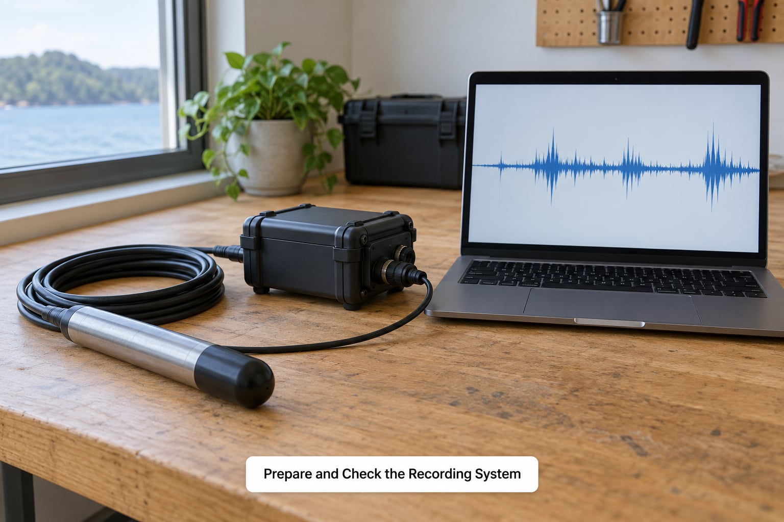
Run the whole chain on a bench before the water touches it. Most field faults are detectable in ten minutes of dry testing.
- Sampling rate. Set it at least twice your highest frequency of interest, and add margin for the anti-aliasing filter. Recording a 10 kHz band at 96 kHz is common; Nyquist alone is a floor, not a plan.
- Bit depth. 16-bit gives about 96 dB of dynamic range; 24-bit gives roughly 144 dB. At a quiet site the extra range is what keeps ambient noise off the digital noise floor.
- Gain. Set it so the loudest expected event lands below full scale with headroom. Automatic gain control is a trap for long deployments: a pile strike resets the gain and the quiet background that follows is recorded at the wrong level.
- File format. Record raw linear PCM. Compressed formats throw away exactly the low-level ambient detail you deployed to capture.
- Clock. Confirm the recorder timestamps accurately. Where several units must line up, synchronise to GPS or a shared oscillator, and budget for drift over a long soak.
- Power and storage. Do the arithmetic above, then halve your estimate for the unexpected.
Then the checks that catch real problems. Short the hydrophone connector and confirm the noise floor is low and flat. Tap or rub the diaphragm and confirm the signal moves. Play a low-level tone from an injection and confirm the amplitude you expect at the recorder input. Record two minutes and look at the spectrogram: a clean input is a narrow flat trace with no hum lines at 50 or 60 Hz and its harmonics. Persistent hum means grounding. Intermittent crackle usually means a wet connector. And note the noise floor as a number now, because later you will want to know whether a quiet recording was genuinely quiet or just the instrument talking.
4. Deploy the Hydrophone Safely
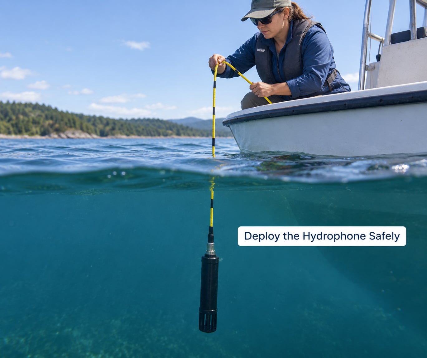
Most ruined recordings are ruined by the deployment, not the sensor. Water moving over the diaphragm generates its own noise, and at flow speeds of one or two knots that noise can exceed a distant source by tens of decibels.
| Method | Best for | Power and data | Typical duration |
|---|---|---|---|
| Moored, bottom-mounted | Ambient baselines, long-term biological monitoring | Batteries and internal or acoustic data storage | Days to months |
| Towed array | Mapping noise across an area or along a track, vessel signatures | Ship power, data logged in real time | Hours to days |
| Hull-mounted | Comparing a vessel’s own radiated noise under way | Ship power, real time logging | Continuous while under way |
| Bottom-mounted cabled | Fixed observatory sites with telemetry | Cable power, real time transmission | Continuous |
| Drifting or free-floating | Rapid reconnaissance where deployment is not possible | Batteries, internal storage | Hours |
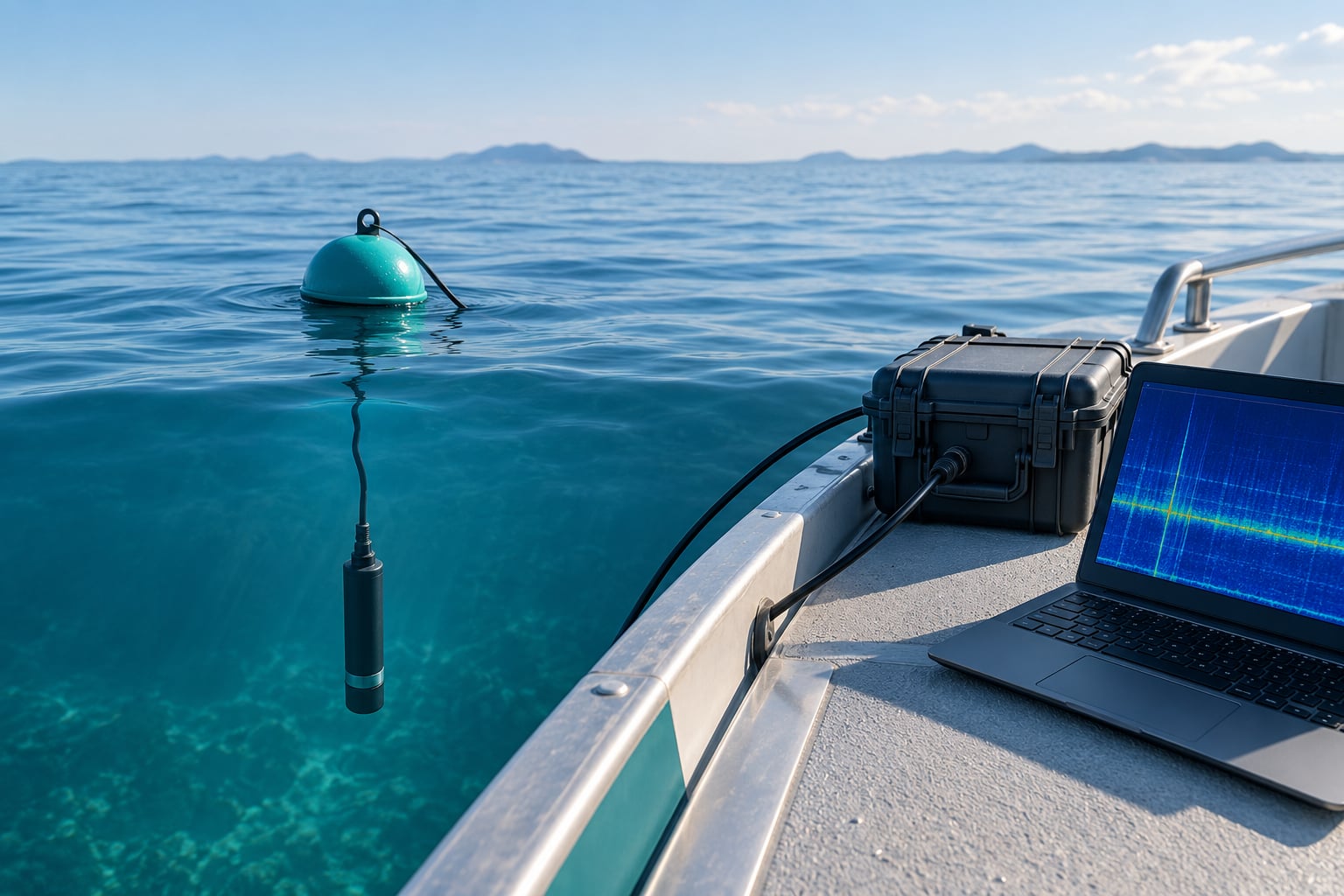
For a mooring, set the sensor in a flow shield or a stilling tube, keep it well below the surface, and make sure the cable is slack and streamed away from the sensor rather than pulled tight above it. A taut cable sings in the current, and the noise it makes looks exactly like a real low-frequency signal until you pull the instrument and it stops. Use a shock absorber between the sensor and the ballast so swell noise does not arrive mechanically. Write down the position, depth, time, weather, sea state and every piece of hardware used, because a month later that log is the only reason the recording can be reused.
Keep the sensor away from the surface unless surface noise is your target. Within a metre or two of the surface, wind, breaking waves and boat wash dominate, and a nearby vessel’s propeller bubble can block your view of everything else. Below that layer the picture is far more stable.
5. Record Ambient and Event-Based Noise
Ambient recording is about characterising the background so you can say whether a source is audible over it. It needs duration rather than intensity: cover at least a full tidal cycle, and preferably a week, so that wind events, spring tides and traffic peaks are all represented in what is otherwise a small sample.
Event-based recording is about a specific source. Keep the instrument in exactly the same place and configuration as the baseline so the two are comparable, note the time of every event in a log, and record a long enough window before and after the event to capture the background. Sliding the sensor a few metres between the baseline and the monitoring run changes your depth and your local multipath, which quietly invalidates the comparison.
Run a calibration tone at the start and end of every deployment rather than trusting the instrument’s certificate from last year. Keep the environmental metadata live: temperature, salinity and depth feed the sound speed calculation used for range and travel time, and a drifting or unlogged sensor cannot be corrected afterwards.
If the deployment is unattended, think about retrieval before you deploy. Data recovery options run from pulling the instrument to acoustic release, surface buoys with an acoustic modem, and satellite uplink for near-real-time reporting. Each adds a failure point, and a lost unit carrying three weeks of data is a bad afternoon.
6. Check, Process, and Interpret the Data
Open every recording before you analyse it. Look for clipping at the top of the waveform, which means the gain was too high and the data is unusable for that event. Look for dropouts and gaps, which point to power or storage faults. Look at the spectrogram: continuous lines at 50 or 60 Hz and their harmonics mean electrical pickup, a broadband smear that moves with the tide is usually flow noise, and regular vertical streaks every few seconds are often cable or mooring strumming.
Then convert volts into level. Add the calibrated receive sensitivity, the preamplifier gain, and any insertion loss, then express the result as decibels referenced to 1 micropascal. A common mistake on DIY builds is to fall back on the air reference of 20 micropascals out of habit, which shifts every number by about 26 dB and makes your data incomparable to anything published.
Read the spectrogram as a picture of level against time and frequency. Low-frequency energy that rises and falls slowly with the tide is probably ambient sea state. Narrow horizontal lines at specific frequencies are tonal sources such as machinery or propeller harmonics. Broadband vertical events that cut off cleanly are impulsive, which is what a pile strike looks like. Step changes that never revert are a settings change by someone on shore.
For reporting, compute broadband levels and octave or one-third octave band levels over fixed intervals, typically one second or one minute, then separate ambient from event. Underwater measurements are not weighted with A-weighting the way airborne measurements are; A-weighting was designed around human hearing in air and has no justification here. If a client asks for dB(A) underwater, it is worth explaining that before producing the number.
One limit worth stating plainly: a single hydrophone measures level, not direction. Working out where a sound came from needs an array, time-of-flight maths and a sound speed profile. A lone sensor tells you how loud and when, which answers most questions people actually ask of it.
Common Mistakes When You Measure Underwater Noise
Flow noise over the diaphragm. The most common fault by a wide margin. It rises with current speed and makes quiet water sound busy. Fix it with a flow shield or stilling tube, test at the deployment site with a hand-line check, and if the spectrum brightens during deployment, that is the cause rather than a real event.
Cable strumming. A taut cable pulled by a slow current produces a low-frequency tone that masquerades as a distant source. Add slack, use a shock absorber, and re-record from a second position to check whether a detection follows the sensor or stays put.
Surface splash and wind noise. Both flood the record with broadband energy. Deploy deeper, below the bubble and wind layer, and record surface conditions in the log so a bad afternoon can be explained later.
Ignoring the self-noise floor. If the ambient level sits at or near the instrument’s noise floor, you are measuring the instrument. Take a noise-floor reading with the hydrophone shorted or acoustically decoupled and compare it against the ambient recording before drawing any conclusion.
Automatic gain and compression. Both look helpful and both destroy the baseline. Fix the gain once, check the headroom, and leave it alone.
Clock drift and unsynchronised units. Two units a few seconds apart will not line up a passing call, and a month of drift will scramble a tidal analysis. Sync to GPS, log the sync procedure, and state the expected drift in the write-up.
Forgetting what the numbers are referenced to. Underwater levels are dB re 1 micropascal. Air dB and air dB(A) are different quantities and cannot be mixed in.
Calibrating once and hoping. Sensitivity shifts with temperature, depth and time, and connectors corrode. A tone at the start and end of the deployment turns a guess into a bounded range.
Frequently Asked Questions
How to measure sound underwater?
Use a hydrophone, a transducer that converts acoustic pressure in water into voltage. Pass that signal through a low-noise preamplifier, digitise it at a sample rate at least twice your top frequency of interest, and record it as linear PCM. Calibrate the chain with a pistonphone or reference transducer at the start and end of the deployment, then convert volts into decibels referenced to 1 micropascal. Read the result as a spectrogram and as octave band levels.
Can humans hear underwater?
Only partially, and badly. Water and body tissue are close enough in density that sound crosses into your body, where bone conduction lets a faint rumble reach the inner ear. But the outer ear is flooded and there is no airborne reference, so you lose the cues that let you localise a sound. Divers describe pressure sensations and low-frequency vibration rather than anything you would call hearing.
What type of noise is underwater?
Natural sources include breaking waves, wind-driven surface noise, rain, biological calls from whales, fish and crustaceans, ice movement, and earthquakes. Human sources include commercial vessel traffic, outboard motors, pile driving, dredging, wind farm construction, seismic surveys and machinery discharge. Natural energy concentrates at low frequencies, while shipping and construction add strong low-frequency tones and broadband energy that overlaps the marine mammal band.
How can noise levels be measured?
A hydrophone measures sound pressure, expressed as decibels referenced to 1 micropascal, which is the underwater standard. For biological effects, some studies also measure particle motion with accelerometers, since low-frequency sound is often detected first by fish and invertebrates. Long deployments need automated quality control: IOOS QARTOD publishes a manual for real-time quality control of passive acoustics observations.
Do hydrophones need calibration?
Yes, and the reason is not fussiness. The recorder measures volts, not pascals, so a sensitivity figure is the only bridge between the two. Without it your data is internally consistent but not comparable to anything. A pistonphone check before and after a deployment gives a bounded sensitivity and lets you state an honest uncertainty, which is what separates a screening record from a defensible one.
How far can a hydrophone hear?
Distance is not a fixed property of the sensor. It depends on source strength, geometric spreading, absorption, the ambient background, and the self-noise floor of your instrument. Low-frequency energy can travel tens of kilometres in seawater, while frequencies of a few kilohertz are absorbed within a few hundred metres. Source level and the SNR you need to beat decide the practical answer.
Start With a Reproducible Baseline
Start here: write the objective as one sentence with a number in it, then bench-test the entire chain and record your instrument’s noise floor as a number. That single habit of measuring your own floor before you go looking for quiet is what separates a recording you can interpret from one you can only look at.
Then run one short, fully documented deployment at a site you can return to. Twenty-four hours is enough to expose flow noise, surface contamination, gain mistakes and clock problems before you commit a month of data to them. Keep the log, keep the raw files, keep the calibration tone, and write the processing chain down as you go. That is what makes the baseline worth something in 2026: someone else can repeat it and get comparable numbers.
Once that first run behaves, extend to a full tidal cycle, add event windows around whatever you are trying to detect, and calibrate at both ends of every deployment. If your measurements ever need to satisfy a regulator or a published study, that is the point at which a traceable instrument and a documented uncertainty budget stop being optional.