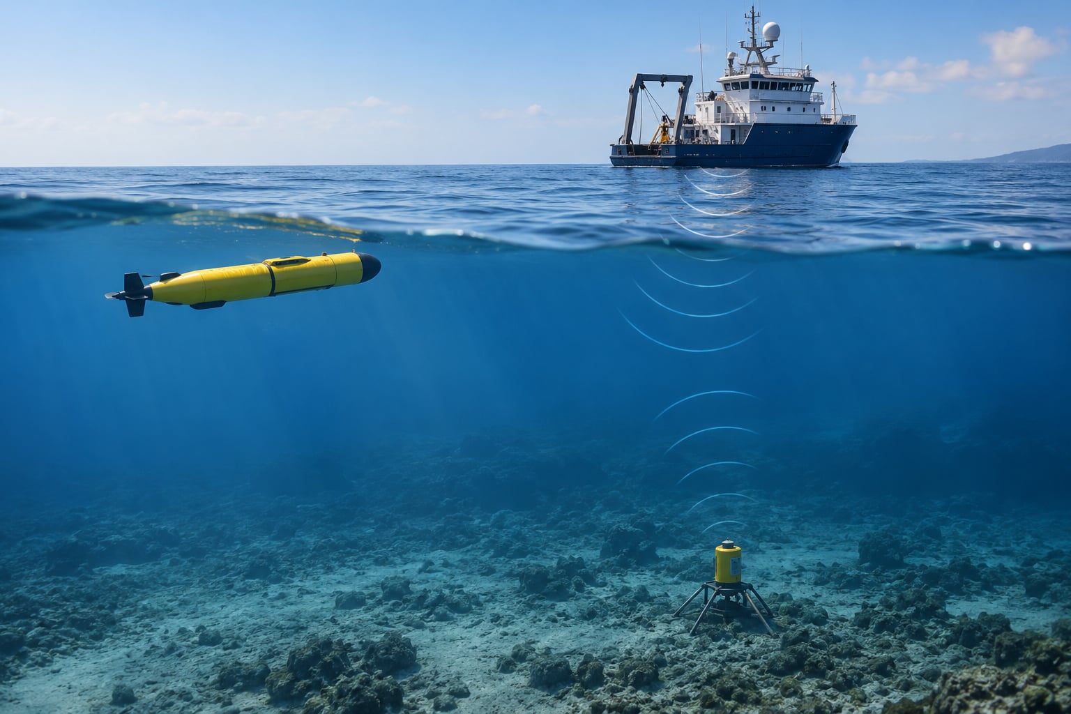
Here is how acoustic positioning works in outline: a sound pulse goes from a reference point at a known location to a transponder on the vehicle, the system times how long it takes to arrive and reply, and that travel time becomes a distance. Several distances combined give the vehicle’s location, in the same way a satellite fixes a phone above water. Underwater, sound is the only signal that travels far enough to do the job, because radio waves and GPS die at the surface.
That is the whole idea in two sentences. The interesting part is what happens between the pulse and the fix, and why the same system behaves very differently at 5 metres in a harbour and 3,000 metres in the North Sea.
This guide covers the mechanism, the system types, the error budget and the practical choices for anyone building an ocean robot. It is written for marine engineers, AUV and ROV operators and makers who already know what a transducer is.
Table of Contents
- How Acoustic Positioning Works: The Basic Idea
- The Components of an Underwater Acoustic Positioning System
- How Underwater Sound Carries a Position Fix
- Why Positioning Uses Two or More Measurements
- Common Acoustic Positioning Methods
- How Environmental Conditions Affect the Result
- How Errors Accumulate in an Acoustic Position Estimate
- How to Choose an Acoustic Positioning Approach for a Sailing Robot
- How Acoustic Positioning Fits Into a Complete Navigation System
- Frequently Asked Questions
- How accurate is acoustic positioning for underwater robots?
- Can acoustic positioning work when GPS is unavailable?
- Why does water depth affect acoustic positioning accuracy?
- How far can an underwater acoustic signal travel?
- What is the difference between USBL and LBL positioning?
- What happens if an underwater acoustic beacon is lost?
- Conclusion: Start With the Positioning Requirement
How Acoustic Positioning Works: The Basic Idea
Underwater acoustic positioning is a method of tracking and navigating vehicles and divers by measuring acoustic distance, direction, or both, then converting those measurements into a position estimate. The reference side of the system sits somewhere with a known location: a survey ship, a moored transponder, or a network of seafloor units.
The target side is a transponder or transceiver bolted to the vehicle. The system measures how long sound takes to travel between them, which gives range. Where the hardware can also work out direction, it gives bearing as well.
Three things get confused with this all the time, so it is worth separating them.
Positioning is not communication
An acoustic communication system sends data: images, telemetry, commands. A positioning system measures time and phase. Many modern units do both in the same exchange, because the reply that carries the position message is already the reply being timed. The signal is doing two jobs at once, but the useful measurement is still the clock.
Positioning is not obstacle avoidance
Obstacle avoidance is local. A sonar looks ahead a few metres and looks for something in the way. Positioning is global: it tells the vehicle where it is in the world, which usually means where it is relative to something that never moves, or relative to a ship whose position is known.
Positioning is not inertial navigation
An inertial navigation system integrates acceleration and rotation to dead-reckon a position. It never gets told where it is; it just keeps adding up the motion. That is why it drifts. Acoustic positioning is the periodic correction that stops the drift, and in practice the two are never used without each other.
The Components of an Underwater Acoustic Positioning System
A working system is more than a transmitter and a receiver. Here are the parts you actually have to specify.
- The surface reference. A transceiver on a vessel, an anchored buoy, or a shore station. In USBL it carries a hydrophone array; in LBL it may be nothing more than an interrogator that pings each seafloor transponder in turn.
- The transponder or transceiver on the vehicle. It listens, and when it hears its own code, it replies. Modern units can also send data back in that reply.
- The transducer. The part that turns electrical energy into pressure waves. Its frequency and its size both matter: small transducers tend to be higher frequency, which travels further through data but not as far through water.
- The hydrophone array. A set of receivers spaced a known distance apart. The spacing is the baseline, and it is what lets the system work out bearing by comparing arrival times across channels.
- The modem and signalling layer. The code that decides which transponder answers, what the reply contains, and how the exchange is kept clean in a busy water column.
- The clock. The least glamorous component and one of the biggest error sources. Timing better than a microsecond is what separates a decent fix from a good one.
- The reference platform’s own position. An antenna or GNSS receiver on the surface, plus a heading source and sometimes an IMU, because knowing the hull’s exact position and heading is half of converting a relative measurement into an absolute one.
Some systems compute the fix on the vehicle and transmit the answer up. Others compute everything remotely at the surface. Both work; the difference matters for bandwidth and for what happens when the link drops.
How Underwater Sound Carries a Position Fix
How acoustic positioning works, step by step
- The interrogator transmits. A surface unit sends a coded acoustic pulse, usually in a narrow frequency band so it can be told apart from noise and from other traffic.
- The transponder hears it. Only the transponder whose code matches replies. This is what lets several vehicles share one water column without all answering at once.
- The reply comes back. Either a second coded pulse or a longer encoded waveform.
- Travel time is measured. Multiply the measured interval by the speed of sound in water and you have a distance. This is time-of-flight ranging, and it is the foundation of everything else.
- Arrival times are compared across the array. In USBL the phase or delay difference between channels tells the system the direction the signal came from.
- Range and bearing become coordinates. The software converts the measurement into an offset from the reference, adds the reference’s own GNSS position and heading, and produces a latitude, longitude and depth.
Higher-frequency systems measure the phase of the returning waveform rather than the round-trip time. Phase is much more precise for short distances, which is why that approach suits a vehicle working close to the array.
Why Positioning Uses Two or More Measurements
One range measurement cannot give you a position. A single distance from a single point describes a circle, and a circle is not a place. Every underwater robot on earth sits somewhere on an infinite number of circles centred on whatever beacon it last heard.
Two ranges from two references narrow it to an intersection point, in the plane, if both references sit at a known depth relative to the vehicle. Three ranges give you a true three-dimensional fix. In practice, depth from a pressure sensor often supplies the third dimension for free, which is why two-beacon systems can still deliver three-dimensional positions.
That geometry is called trilateration when it uses ranges, and triangulation when it uses angles. The distinction matters less to the operator than the resulting sensitivity: with two references the error grows quickly as you move away from the line between them, so geometry matters as much as hardware quality.
One useful way to picture it: if a vehicle drifts directly out along the line joining two beacons, the ranges barely change and the position estimate degrades fast. If it drifts sideways from that line, the ranges change quickly and the fix stays good. Teams that deploy baselines care about that geometry, which is why baselines are laid out in a triangle or rectangle rather than a single straight line where they can.
Common Acoustic Positioning Methods
Four classes cover most working systems. They differ in where the reference sits, how much hardware that takes, and how the position is calculated.
| Method | Where the reference lives | Typical scale | Accuracy | Hardware and deployment | Best suited to |
|---|---|---|---|---|---|
| Long baseline (LBL) | Three or more transponders on the seabed | Kilometres, tied to transponder spacing | Often around 0.5 to 1 percent of slant range | Most deployment work; baseline must be surveyed | Long-duration seabed work, AUV navigation, precision survey |
| Ultra-short baseline (USBL) | Hydrophone array under a vessel or mounted on the hull | Usually a few hundred metres to around a kilometre | Around 0.3 to 1 percent of slant range | One array on one ship; quick to mobilise | ROV tracking, dive supervision, pipeline and cable inspection |
| Short baseline (SBL) | Transponder on a line or on the vehicle itself | Short, often under a few hundred metres | Very high relative accuracy | Simple, often combined with data transfer | Under a pier or a ship, relative tracking between two units |
| GPS intelligent buoys (GIB) | Buoys held at known positions on the surface | Shallow and coastal work | Good relative to surface references | Surface units only, no seabed deployment | Harbour, estuary and shallow-water surveys |
Long baseline systems get their accuracy from geometry: references are far apart, so the circles of uncertainty intersect at a shallow angle and the position is well conditioned. USBL trades that for convenience, squeezing bearing out of a metre-wide array on a moving ship, which means the array has to be calibrated tightly and the ship has to know its own heading well.
Hybrid arrangements exist for the awkward cases. A long-range USBL setup can place a transponder on the seabed and read it with a surface array, extending useful range far beyond what a hull-mounted array can do in noisy water.
It helps to know where each system’s accuracy estimate comes from. Some quote a percentage of slant range, some quote a fixed circle of error at a given depth, and some quote a horizontal figure that quietly assumes a calm sea. Practitioners on industry forums are blunt about this: published accuracy claims rarely survive contact with a working site, and real-world performance in shallow water degrades quickly beyond roughly 100 to 200 metres because of multipath. Put plainly, how acoustic positioning works on a spec sheet and how it works on a boat at sea are often two different stories.
How Environmental Conditions Affect the Result
Water is not a uniform medium. It has a sound speed that varies with depth, and every assumption the timing math rests on depends on knowing what that speed was along the path.
Sound speed and the profile
Typical seawater carries sound at roughly 1450 to 1550 metres per second, and that number shifts with temperature, salinity and pressure. Warm, shallow water is fast; cold deep water is slow. Because sound bends toward slower water, a sound velocity profile can bend a ray that travels far away from the straight line the geometry assumes. Over a long path, an unmeasured profile turns into a real position error.
Frequency and range
Higher frequencies carry more data and resolve phase more finely. They also fade faster with distance. This is the central trade-off in system selection.
| Typical frequency band | What you gain | What you lose | Common working range |
|---|---|---|---|
| Roughly 8 to 15 kHz | Long range, good tolerance of noise | Narrow bandwidth, slow data | Several kilometres in open water |
| Roughly 19 to 36 kHz | Better data rate, tighter phase measurement | Shorter range, more sensitive to surface noise | Around a kilometre or two |
| Roughly 38 to 50 kHz | Fine bearing, compact arrays | Short range | Hundreds of metres |
| Above about 100 kHz | Very fine range and bearing resolution | Very short range, cavitation risk near a propeller | Tens to low hundreds of metres |
Multipath, surface and seabed
In shallow water the surface and the seabed bounce the signal, and the receiver sees several copies of it a few milliseconds apart. The first arrival is the direct path; the rest are echoes. Shallow water is where shallow-water acoustic positioning suffers most, and it is the single most common cause of a fix that looks plausible and is quietly wrong.
Noise and motion
Propeller wash, thrusters, flow noise and even the vehicle’s own motion smear the arrival measurement. A turning propeller is worse than a fast-moving vehicle, which is why a vessel is often asked to slow down or hold a course during a fix.
How Errors Accumulate in an Acoustic Position Estimate
A reported position is never a point. It is a point plus a confidence region, and understanding the region is what makes the number usable.
- Clock error. A microsecond of timing error is roughly a millimetre of range, but real oscillators drift and are affected by temperature.
- Sound speed error. A one percent error in assumed sound speed over a 500 metre path is several metres of position error.
- Receiver geometry. Poorly placed references turn a small range error into a large position error. This is usually the biggest term and the least discussed.
- Attenuation. Weaker signals give noisier arrival estimates, so error grows with range even in clean water.
- Multipath. Echoes bias the timing, and the bias is worse in shallow water and around reflective structures.
- Calibration drift. An array’s phase calibration shifts with temperature and mounting. Re-calibration is part of operating, not a one-off.
- Reference position and heading. If the surface platform’s GNSS fix or compass heading is wrong, the subsea position inherits that error directly.
Good software reports horizontal and vertical error separately, rejects outliers, and smooths rather than filters hard. When a system quietly clamps a bad measurement instead of flagging it, the errors stop being visible, which is worse than having none.
How to Choose an Acoustic Positioning Approach for a Sailing Robot
For an uncrewed surface or subsurface robot, the decision narrows fast once you fix a few numbers.
- Write down the accuracy you need, in metres. Holding a station within two metres and logging a pipeline to within one are very different projects from tracking a vehicle over a few kilometres.
- Measure the water depth and the depth band the robot will work in. Deep water with a hull-mounted array is the hardest case. Baselines on the seabed, or an inverted transponder under a small mooring, usually beat trying to push a surface array down.
- Check what the robot can carry. Power draw and weight are usually the real constraints. A high-frequency array is small and hungry; a long-range unit is bulky.
- Decide how long the mission runs. Minutes next to a support vessel suits USBL. Days on the seabed suits LBL, once you accept the deployment effort.
- Look at what else is on board. If the robot already carries a DVL and an IMU, a slower acoustic fix is enough. Without them, you need a faster fix because dead reckoning has nothing to stand on.
- Test the geometry, not just the datasheet. Before you commit, log positions where the vehicle will actually go and check the error ellipsoid along that track.
The tethered case is worth calling out. A fibre or power cable running to a surface unit removes the acoustic link entirely for communication, though it does not remove the need for position fixes on the vehicle. Cables solve power and bandwidth problems and create their own: they constrain depth, they snag, and they turn a free-ranging robot into a tethered one.
How Acoustic Positioning Fits Into a Complete Navigation System
No serious marine robot navigates on acoustics alone. The usual stack layers sensors that each cover the others’ weaknesses.
- GNSS at the surface gives the reference platform an absolute position, accurate to a few metres. It stops at the waterline.
- Inertial navigation bridges the gap between fixes, at the cost of drift that grows with time and motion.
- A DVL measures velocity relative to the seabed and holds altitude at the same time, which is what makes dead reckoning viable over a short mission.
- Pressure and depth supply the vertical dimension cheaply, and often turn a two-dimensional fix into a three-dimensional one.
- Compass and attitude sensors turn relative measurements into absolute ones, and on many vehicles an acoustic-derived heading is the reference everything else is compared against.
- Environmental inputs such as depth, temperature and a sound velocity estimate feed the propagation model that converts travel time into distance.
The fusion rule is simple in principle: trust the acoustic fix when it arrives, coast on the inertial solution in between, and weight the acoustic result by its reported error. Practitioners in the ROV community broadly agree on the pattern of fusing USBL with a DVL and INS, because the errors are independent and the combination holds up far better than either sensor alone.
Frequently Asked Questions
How accurate is acoustic positioning for underwater robots?
Most systems quote accuracy as a percentage of slant range rather than a fixed number, typically around 0.3 to 1 percent for USBL and LBL. At 200 metres slant range, one percent is two metres of error. Real accuracy is usually worse than the datasheet figure in shallow water, where multipath reflections and surface noise dominate, so treat the published number as a best case in good conditions.
Can acoustic positioning work when GPS is unavailable?
Yes, and that is the main reason it exists. GPS and GNSS signals are radio, and radio attenuates sharply in seawater, so a receiver metres below the surface gets nothing usable. Acoustic positioning works entirely within the water column, using sound between beacons that are all underwater, so it needs no satellite signal at all. Only the surface reference needs GNSS, and even that can be tied to a surveyed point.
Why does water depth affect acoustic positioning accuracy?
Depth changes the geometry of the measurement and the environment around it. A deeper target sits further from the surface array and often further from the direct path, so more of the energy arrives as reflected paths off the surface and seabed. Shallow water also allows many more bounces within the system’s listening window, which makes multipath error the dominant term rather than clock or sound speed error.
How far can an underwater acoustic signal travel?
It depends heavily on frequency. Bands in the 8 to 15 kHz range routinely carry a signal several kilometres in open water, while bands above 100 kHz are useful over tens to a couple of hundred metres. Range also falls in noisy or sediment-laden water, and very low frequencies are limited by ambient noise rather than by absorption. Longer range always costs bandwidth, so low-frequency links carry position data rather than video.
What is the difference between USBL and LBL positioning?
USBL takes its bearing measurement from a compact hydrophone array mounted on a vessel or vehicle, so one unit gives you a fix but the array is small and sensitive to calibration and vessel motion. LBL uses three or more widely separated transponders on the seabed, so the geometry does the work and accuracy holds over longer distances. LBL is more accurate and far more work to deploy; USBL is quick to mobilise and suited to short-range tracking.
What happens if an underwater acoustic beacon is lost?
The system notices through missing or inconsistent replies, and the behaviour depends on the architecture. A USBL setup usually just stops updating that vehicle until the signal returns. An LBL system may lose one reference of three and continue on reduced geometry with larger errors, or lose a reference it depends on entirely. Good software reports the loss and the resulting degraded confidence rather than quietly reusing the last known position.
Conclusion: Start With the Positioning Requirement
The first three decisions on any project are the same. How accurate does the position have to be, in metres. Where will the vehicle actually be, in depth and in distance from any surface reference. And what is already on board, because a DVL and an INS change which acoustic system is worth buying.
After that, how acoustic positioning works in the field comes down mostly to geometry. Deploy long baseline if you can afford the work, use ultra-short baseline if you cannot, and always plan the sensor layout around the track the vehicle will fly rather than the map in the abstract.
The practical next step is cheap: pick a stretch of your intended operating area, log fixes along it with borrowed or leased gear, and compare the error ellipsoid against what the mission actually requires. That one afternoon usually answers the question faster than another week of reading specifications.