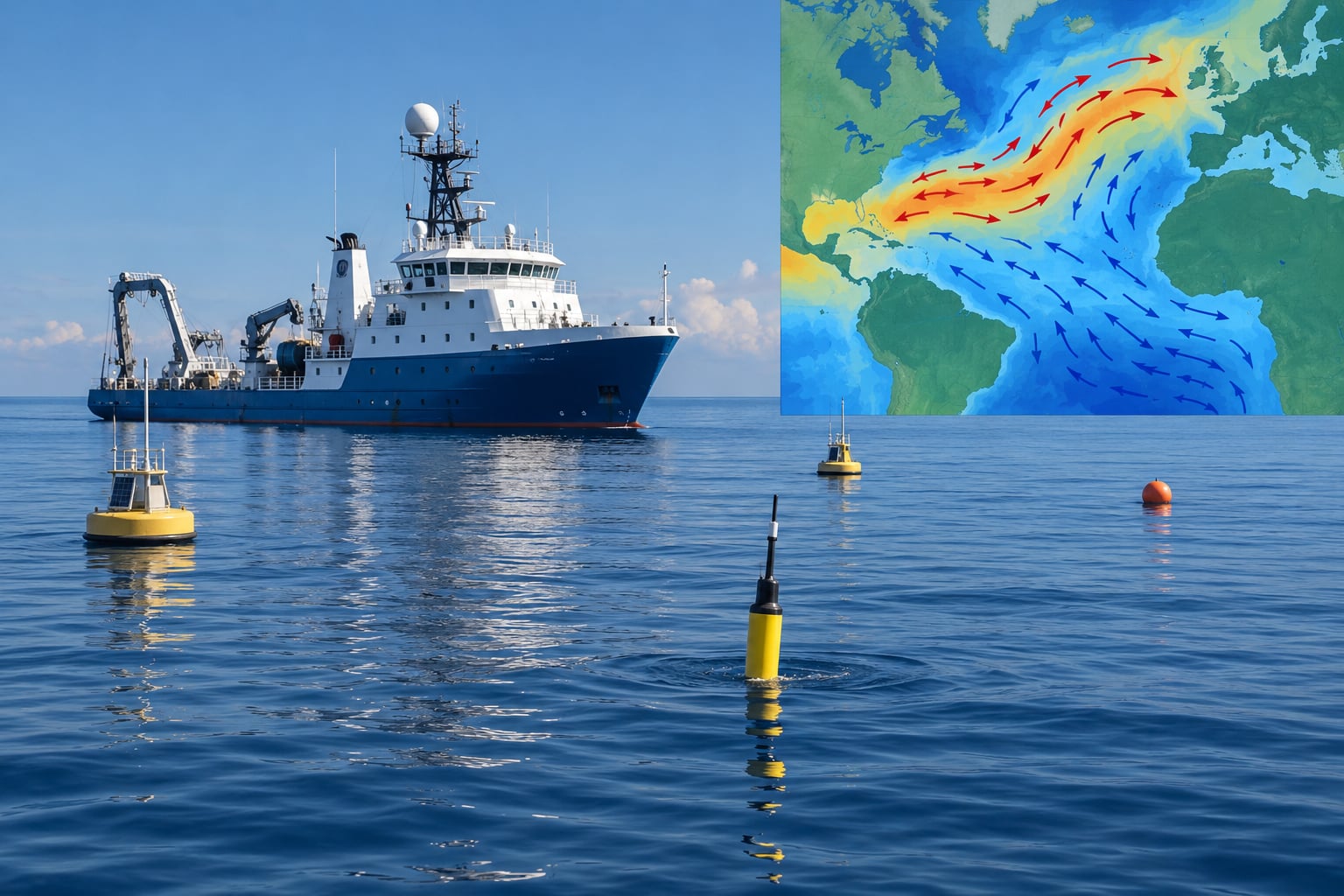
An ocean model forecasts currents by turning the ocean into a grid, filling that grid with the best available real-world measurements, and then stepping the physics of moving water forward in time. Satellites, floats, buoys and radar supply the starting picture; a data assimilation step corrects that picture against reality; the model then runs the equations of motion ahead of the clock. Nothing is guessed from experience alone.
That chain runs quietly in the background of nearly every piece of marine technology. A sailing robot decides which tacking angle pays off. A port operator works out whether a swell will set a vessel onto the berth. A search coordinator asks where a life raft will be at dawn. All of them are reading a current field that a model produced, validated, and published in 2026.
This guide walks that chain end to end, then gets practical about accuracy, resolution and the files you download. I have pulled the specifics from operational centres rather than textbooks, because the interesting details — why a 1/12 degree global model cannot tell you about your harbour, why day three is fine offshore and useless in an estuary — live in the operational systems.
Table of Contents
- What Does an Ocean Model Do?
- How Ocean Models Forecast Currents
- What Data Goes Into a Current Forecast?
- How Physics and Computer Grids Work Together
- What Are the Main Forecasting Methods?
- How Do Researchers Check Whether a Forecast Is Accurate?
- What Causes Uncertainty in Current Forecasts?
- How Are Current Forecasts Used in Marine Technology?
- Frequently Asked Questions
- How far ahead can ocean models forecast currents?
- Do ocean models predict currents better than waves?
- Why do current forecasts change after new satellite or buoy data arrives?
- What is data assimilation in ocean current forecasting?
- Are ocean current forecasts accurate near coastlines?
- How do autonomous sailing robots use current forecasts?
What Does an Ocean Model Do?
An ocean circulation model is a computer program that divides the ocean into a three-dimensional grid, solves the equations of motion for every cell, drives them with wind, heat and river inputs, and repeatedly nudges the simulated state toward real measurements so its output tracks the actual ocean instead of drifting away from it.
Those four elements — grid, equations, forcing, assimilation — are the whole architecture. The grid is the discretisation: horizontal cells a few kilometres or smaller, stacked into vertical layers that are thin near the surface and the sea floor and thicker in between. The equations are the fluid dynamics, in practice a simplified form known as the primitive equations that assumes pressure varies vertically but not horizontally.
The forcing is everything the ocean cannot work out on its own. Wind stress is usually the largest single driver of the upper ocean. Heat flux, precipitation, evaporation, cloud cover, river discharge and tides all push on the model from outside. And the assimilation step is the correction loop: every forecast cycle, the model’s own state is nudged toward whatever the satellites, floats and buoys actually reported in the last few hours.
What comes out the far end is a gridded field of velocity — typically in metres per second — at each depth and each time, alongside temperature, salinity, sea surface height and, in coupled systems, waves. It is a description of a moving fluid across an entire region, not a reading from one point.
How Ocean Models Forecast Currents
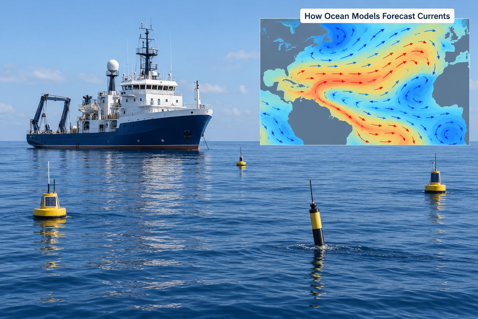
Every operational forecast you can download is the output of the same six-step cycle, repeated several times a day. The steps matter more than the individual models, because a beautiful model with a poor starting state produces a confident wrong answer.
1. Observe
Satellites, moored buoys, drifting buoys, profiling floats, high-frequency radar, ships and tide gauges report what the ocean is doing right now. Each has gaps, so no single instrument covers the picture. The observing network is assembled specifically so that the gaps in one source are filled by another.
2. Assimilate
All those observations are folded into the model to correct its state. This is the step that separates a forecast from a guess, and the one most often named without explanation. In plain terms, the model takes a first guess at the current state, compares it against what the instruments reported, and shifts the fields to reduce the mismatch — without destroying the balance the physics requires.
3. Initialise
The corrected state becomes the starting point, or initial condition, for the forecast run. It also usually needs a spin-up period first: the model is integrated over weeks or months with the observed forcing so the water column settles into a realistic state instead of starting from a static ocean.
4. Integrate forward
Now the model runs. At each time step the code computes how momentum, heat and salt move through every cell, using the atmosphere’s forecast as its boundary condition. The model is not looking up an answer; it is solving the same physics that produce the real current, thousands of steps per simulated day.
5. Validate
Forecasters withhold some observations from the assimilation and score the run against them. If a model systematically gets the same places wrong, that pattern is fed back into the system — into physics, parameterisations, bias correction — rather than ignored.
6. Publish
The fields go out as gridded files, usually NetCDF or GRIB, on a regular grid with a time axis. NCEP’s Global RTOFS and the Copernicus Marine Service publish exactly this way, and a small regional centre such as Ireland’s Marine Institute ships hourly surface current fields in GRIB over FTP.
What Data Goes Into a Current Forecast?
The data going in determine the data coming out. Each source measures something different, and operational systems are assembled so that no single failure mode can blind the model.
Satellite altimetry measures sea surface height along repeat orbital tracks. It gives an indirect but wide view: where the sea surface tilts, geostrophic balance puts a current nearby. The trade-off is that altimeters resolve the surface expression, not the current itself, and the tracks are far apart between satellites. The newer SWOT satellite adds much finer along-track resolution in coastal and shelf water, which is precisely where older missions were weakest.
Argo profiling floats drift, sink to about 2,000 m, and measure temperature and salinity on the way back up. They do not measure velocity at all, but temperature and salinity define density, and density gradients set the baroclinic pressure field that moves the deep water. The global array is the backbone of the free-ocean observing system.
Buoys and moorings carry current meters, often acoustic Doppler current profilers, or ADCPs, that measure speed and direction directly through the water column. A mooring holds position so it gives a long, clean time series at one place. The limitation is coverage: each buoy is one point, and there are not many of them.
High-frequency radar maps the near-surface current field over a coastal strip of tens of kilometres, updating every few minutes. This is the highest-temporal-resolution current data anywhere, and it is the reason harbour approaches and straits are now forecast at all. It costs a lot per installation, so coverage is patchy.
Surface drifters measure the velocity of the water they float in, and the surface velocity they report approximates the top few metres. Cheap, numerous, and directly relevant to a sailing robot or a spill. Their weakness is that the wind blows them around, so they need a wind correction and they sample the surface rather than the subsurface.
Ship-based instruments — ADCPs mounted on the hull, thermosalinograph intake lines, and underway CTD casts — turn research vessels and some commercial ships into moving sensor platforms. Coverage follows the shipping lanes rather than the science question, which is a limitation everywhere and an advantage in busy waters.
Tide gauges measure sea level at fixed coastal points. They are long, well-calibrated records, and they constrain the tidal signal that has to be removed before a forecast current can be called a net current.
Then there is the static and the atmospheric input: bathymetry, which sets where the water is squeezed; river discharge; tide constituents; and atmospheric forcing from a numerical weather prediction model — wind, heat, precipitation, evaporation and cloud. DFO describes that last input plainly as the conditions the surface is exposed to, and it is fair to call it the dominant control on the upper ocean.
How ocean models forecast currents across scales
No instrument covers every scale, and that is not a gap anyone is closing. The altimeter sees a basin. The radar sees a coast. The buoy sees a point. A current forecast is a blend, and the blend is weighted by what the model must get right for the job at hand — basin-scale routing, shelf currents, or the set of a mooring in a channel.
So the honest answer to how ocean models forecast currents at any given spot is that you get the best of what is in range. Offshore, the altimeter and Argo dominate and the field is trustworthy over days. In a strait, the radar and a moored ADCP dominate and the field is trustworthy over hours.
How Physics and Computer Grids Work Together
Water in the ocean is pushed around by four things: the pressure gradient, which sends water from high sea level to low; the rotation of the Earth, which deflects that flow into a geostrophic balance where the current runs along contours of constant pressure; gravity acting on density differences, which drives the deep thermohaline circulation; and friction, from the sea floor, the surface and the turbulence inside the water column.
Models get the geometry right by simplifying. Most ocean models assume hydrostatic pressure — the ocean’s pressure changes with depth but hardly at all sideways — which allows the equations to be solved much faster, and use a Boussinesq approximation that treats seawater as incompressible. The cost is that any process requiring the horizontal pressure gradient to be resolved exactly, such as internal waves, is left out of the momentum budget.
On top of that sits turbulence. The ocean mixes itself through convection, wind stirring, internal wave breaking and bottom friction, and the grid cannot resolve any of that at centimetre scale. Models therefore use a turbulence closure scheme plus parameterisations — for example, a bottom roughness parameterisation that turns a rough sea floor into an effective drag. Dynamic vegetation drag is a newer one: kelp and seagrass beds slow the flow above them, and getting that wrong puts a forecast’s bottom layer in the wrong place.
The grid and the time step are linked. A finer grid resolves shorter waves, so the time step must shrink to keep the integration stable. That is why resolution is expensive: roughly, halving the cell size multiplies the compute by a factor of eight in three dimensions. This is the single biggest reason a harbour-scale forecast needs a dedicated model rather than a zoomed global one.
Regional models handle scale by nesting. A one-way nested coastal run takes its boundary values from a parent global model and refines the interior, which is cheap and safe but cannot send anything back. Two-way nesting, as in the NEMO-AGRIF scheme, lets the fine grid feed the coarse grid and capture the effect of a headland on the basin. Many centres also use unstructured grids, which concentrate resolution exactly where the coastline demands it.
What Are the Main Forecasting Methods?
Five families of method produce the currents you actually see on a chart, and they differ in what they can and cannot do.
Persistent forecasts assume today’s current keeps going. They are surprisingly hard to beat at day one, and useless past a few days. Their real value is as the baseline every other method must beat to prove skill.
Statistical and harmonic models predict tidal currents from the astronomical constituents. Tides are deterministic, so this works to remarkable accuracy over years — the Irish Marine Institute publishes tidal predictions for around 40 locations on a two-year horizon. Statistical regression adds a wind-driven and seasonal component, and remains common for port approaches because it is cheap and fast.
Hydrodynamic models solve the equations of motion on a grid. This is where the non-tidal current lives, and where a proper forecast is won. They carry tides naturally, which is what separates them from a pure statistical model.
Data assimilation is the layer that turns a simulation into a forecast. It is worth being precise about the vocabulary: the first guess is the background field, the model state before correction; the observation operator maps the model state to what each instrument would have measured; the difference between the two is the innovation; and the analysis is the corrected field that gets integrated forward. Three-dimensional variational schemes adjust the whole water column at once, so a single sea surface height observation constrains a subsurface structure rather than just the surface.
Coupled systems run ocean, atmosphere and sea ice together, so the surface currents respond to the weather model’s own heat and momentum fluxes rather than to a separate forcing product. DFO and the Marine Institute both describe coupling as the direction of travel, and it is the standard for storm surge and marine heatwave work.
Ensembles and machine learning address uncertainty. Running the same model several times from slightly different initial states shows how much the answer depends on the starting picture, which is the honest way to publish a confidence range. On the machine learning side, the published results split into three uses: deep autoregressive networks that predict currents in real time from sparse observations, convolutional networks that downscale coarse sea surface height fields into fine current fields, and learned subgrid parameterisations that stand in for turbulence the grid cannot resolve. A hybrid, loosely observed region is exactly where these earn their place, and all three remain research tools rather than operational replacements.
| Model | Typical resolution | Typical use | Runs in |
|---|---|---|---|
| HYCOM | 1/12 degree global, roughly 8 km at the equator | Global analysis and forecast, coupled with sea ice | NCEP Global RTOFS, US Navy |
| NEMO | 1 degree global down to regional kilometres | Global and regional ocean-atmosphere-ice forecasting, climate | Copernicus Marine, CMIP6 |
| ROMS | Regional, hundreds of metres to a few kilometres | Coastal and regional research, nested setups | Universities and research centres |
| CROCO | 1-2 km regional, often with biogeochemistry | Shelf and coastal operations, water quality | Marine Institute, Mercator Ocean partners |
| NEMO-AGRIF | Regional to coastal refinement | Two-way nested coastal systems | Copernicus coastal services |
Two of these are worth knowing in detail. Global RTOFS runs the US Navy implementation of HYCOM with a data assimilation system, giving a global current analysis at 1/12 degree alongside the forecast. The Copernicus Marine Service distributes regional and global products built on NEMO, with a public catalogue you can browse and subset without institutional access. Both are free, and both are a better answer to “what app should I use” than any consumer weather app.
How Do Researchers Check Whether a Forecast Is Accurate?
A forecast nobody scores is a forecast nobody should use. The standard method is simple: hold out some observations, run the forecast without them, and compare the model against what actually happened.
The common measures are root mean square error for magnitude, mean absolute error when outliers should count less, correlation for pattern agreement, and vector error for currents, which are two-dimensional and can be right in speed but wrong in direction. None of them is sufficient alone. A model that predicts zero current everywhere has zero error and no skill, which is why a forecast is always scored against a baseline — usually persistence — and reported as skill relative to that baseline.
What the numbers show in practice is worth stating plainly. In a HYCOM user forum thread, practitioners comparing their own tidal elevation statistics found a mean M2 RMS error of 8.3 cm at 102 pelagic tide gauges for a non-assimilative configuration, against about 1.5 cm for data-assimilative runs. That is a five-fold difference, and it came from the assimilation step rather than from a better grid.
Errors also grow with lead time, and how fast depends almost entirely on the place. A summary of useful horizons:
| Use case | Reliable lead time | What controls it | Model scale needed |
|---|---|---|---|
| Open-ocean routing | 3-5 days | Slow-moving mesoscale eddies | 1/12 degree global or better |
| Shelf and coastal routing | 1-3 days | Mesoscale variability and surface forcing | 1 km or finer |
| Berth, mooring and tug planning | 6-24 hours | Tides, wind and river input | Regional to port scale |
| Estuary and harbour current | Hours | River discharge, wetting-drying, wind | 1-10 m grid |
Two things make coastal and estuarine forecasting harder. Tidal asymmetry means the flood and ebb currents do not mirror each other, and a scheme tuned in a micro-tidal coast will not transfer to a meso- or macro-tidal one — which is part of why data assimilation is so much harder in meso- and macro-tidal regions. And the binding constraint is often not the ocean model at all: operational atmospheric forcing runs at roughly 2-5 km resolution, so however fine your coastal grid is, the surface stress driving it arrives at a coarser scale than you would like.
Intercomparison is the check on the whole field. When five European systems were run over the same Storm Gloria event in January 2020 and compared against each other and against observations, the spread between them was as informative as the comparison to reality. Agreement raises confidence; disagreement is itself a forecast product.
What Causes Uncertainty in Current Forecasts?
Uncertainty in current forecasts comes from six sources, and knowing which one is biting tells you what to do about it.
The initial state. This is the dominant term, and a research audience put it better than any textbook: a forecast is highly sensitive to how good the initial state is, so a bad initial state produces bad later states no matter how good the model is. Errors double roughly every day as the model drifts from truth, and the rate depends on how fast the ocean is changing.
Unresolved small-scale physics. Eddies and fronts narrower than a cell are parameterised rather than simulated. In energetic regions that substitution is a large error source, and it is one reason bias correction and AI-based subgrid schemes are active research areas.
Observational gaps. Between satellite tracks, outside radar coverage and away from moorings, the assimilation has nothing to constrain it. A system can only be as good as the network feeding it, which is why HF radar installations and SWOT coastal altimetry improve models as well as being products in their own right.
Boundary conditions and forcing. River discharge is measured rather than forecast, so a rainy week upstream degrades an estuary forecast before the storm even reaches the coast. Bathymetry errors shift where the flow squeezes, and a wrongly shallow bank puts an eddy in the wrong place.
Systematic model bias. Coastal models are known to be too energetic or too smooth in predictable ways, driven by surface forcing errors, vertical mixing parameterisations, and light attenuation assumptions that matter wherever a model carries biogeochemistry. In shallow, strongly tidal water these biases are not noise; they are the difference between a usable berth forecast and a wrong one.
Resolution mismatch. The most common user error is not a bad model but an unsuitable one. A 1/12 degree global model cannot represent your harbour, strait or estuary. Below the resolvable scale a model is not merely less accurate — it is structurally unable to answer the question, and no amount of skill scoring will change that.
How Are Current Forecasts Used in Marine Technology?
For a robotics or sensor build, the practical question is what the model actually ingests, because that is the measurement that earns its place on the platform. An ADCP mounted on a mooring or a hull is directly assimilated. A CTD or temperature chain feeds the density fields that set the deep circulation. A surface drifter feeds the surface layer a sailing vehicle cares about most. HF radar data is assimilated within its coverage footprint. Knowing this turns a sensor choice from a guess into a contribution.
Autonomous sailing robots use current fields as a cost term in route planning rather than as a hazard warning. A sailboat that understands the tidal stream at a strait can time its transit instead of fighting it. The Marine Institute publishes hourly surface current fields in GRIB specifically for this kind of use, and the whole loop closes when the robot’s own ADCP measurements are later assimilated back into a regional model.
Autonomous ocean drones use the same fields for two purposes: where to steer to catch a feature, and how to interpret what the sensor recorded. A profiler that knows the eddy was expected can separate real signal from instrument drift.
Port and route planning uses the tidal and net components separately. A tidal current reverses on a known astronomical schedule; a net current is the residual that does not. For berthing, what matters is the set and drift through the whole tidal cycle, so tidal streams are added to the net field rather than treated as noise. Marine Institute operational figures illustrate the trade-off: 2 km ocean forecasts run to about three days, 1.8 km wave forecasts to about six.
Search and rescue and oil spill response treat the current field as a spreading model. Both need the same three days of useful lead time, and both are the use case where honest error bars matter most, because a decision to launch happens early.
Environmental and industrial uses include dredging and sediment transport, fish farm siting, harmful algal bloom bulletins driven by a coupled CROCO configuration with PISCES biogeochemistry, and marine heatwave early warning, where the forecast is run ahead of the season rather than the weather.
Finally, how to read what you downloaded. Files arrive as NetCDF or GRIB, and the first thing to check is units: some fields are metres per second, others centimetres per second, and a factor of one hundred is an easy and total mistake. Then decide whether you have a net current or a tidal one, and whether the field is depth-averaged, surface, or a specific layer. Sea surface height anomaly maps convert to current through geostrophic balance, which is fast and free, but it describes only the balanced part of the flow. And read the metadata date: a model field is a snapshot of a cycle, not a live observation.
Frequently Asked Questions
How far ahead can ocean models forecast currents?
Useful lead time depends almost entirely on where you are. In the open ocean, current fields stay useful for about three to five days, because mesoscale features move slowly. On the shelf and near the coast, expect one to three days. Inside an estuary, a harbour or a berth, the honest answer is hours, since tides, wind and river discharge change the answer faster than any global model can track. Always match the model scale to the place before trusting a lead time.
Do ocean models predict currents better than waves?
Waves, usually. Wave height and period respond to wind over relatively short fetch and travel quickly, so a wave model stays accurate much further ahead than a current field. Currents integrate momentum over weeks and months, so they depend on the whole prior history of the water column, and their error compounds. A day-five wave forecast is routinely better than a day-five current forecast for the same location.
Why do current forecasts change after new satellite or buoy data arrives?
Because every forecast run starts by correcting the model state against real observations, and a new altimeter pass, Argo profile or radar snapshot changes what the model believes the ocean is doing now. Data assimilation adjusts the whole three-dimensional field to fit the new data, so the entire forecast shifts, not just the values near the instrument. This is why two runs for the same valid time can differ, and why later cycles usually win.
What is data assimilation in ocean current forecasting?
Data assimilation is the step that folds real measurements into a model before it runs ahead. The model produces a first guess, called the background field, and an observation operator works out what each instrument should have measured. The difference between the two is the innovation, and the analysis is the corrected state that reduces the difference while keeping the physics balanced. Without it you are extrapolating a simulation, not forecasting the ocean.
Are ocean current forecasts accurate near coastlines?
Less accurate, over a shorter horizon, and for a structural reason rather than a tuning failure. A global model at 1/12 degree has cells of roughly eight kilometres, so it cannot represent a harbour, a strait or an estuary at all. Coastal systems run at about 1 km or finer, with the important caveat that atmospheric forcing is only 2-5 km, which caps realism. Below the resolvable scale a model is not merely less accurate, it is unable to answer the question.
How do autonomous sailing robots use current forecasts?
They treat currents as a routing cost, not a hazard. A robot that knows the tidal stream through a strait can time its transit to ride the flood rather than fight it, and can plan tacking angles that account for a steady set across the rhumb line. They read gridded current fields, usually GRIB, and blend them with their own ADCP measurements. Those measurements are then often assimilated back into the regional model, closing the loop.
Start with two habits. First, go and look at the data yourself: NCEP Global RTOFS and the Copernicus Marine Service both publish current analyses and forecasts free to anyone, and reading a real field teaches more in an hour than any description. Second, know the resolution and the lead time before you plan around a forecast. Match the model to the water you are in, treat the first two days as dependable and everything after as guidance, and prefer the product whose resolution actually fits your site.