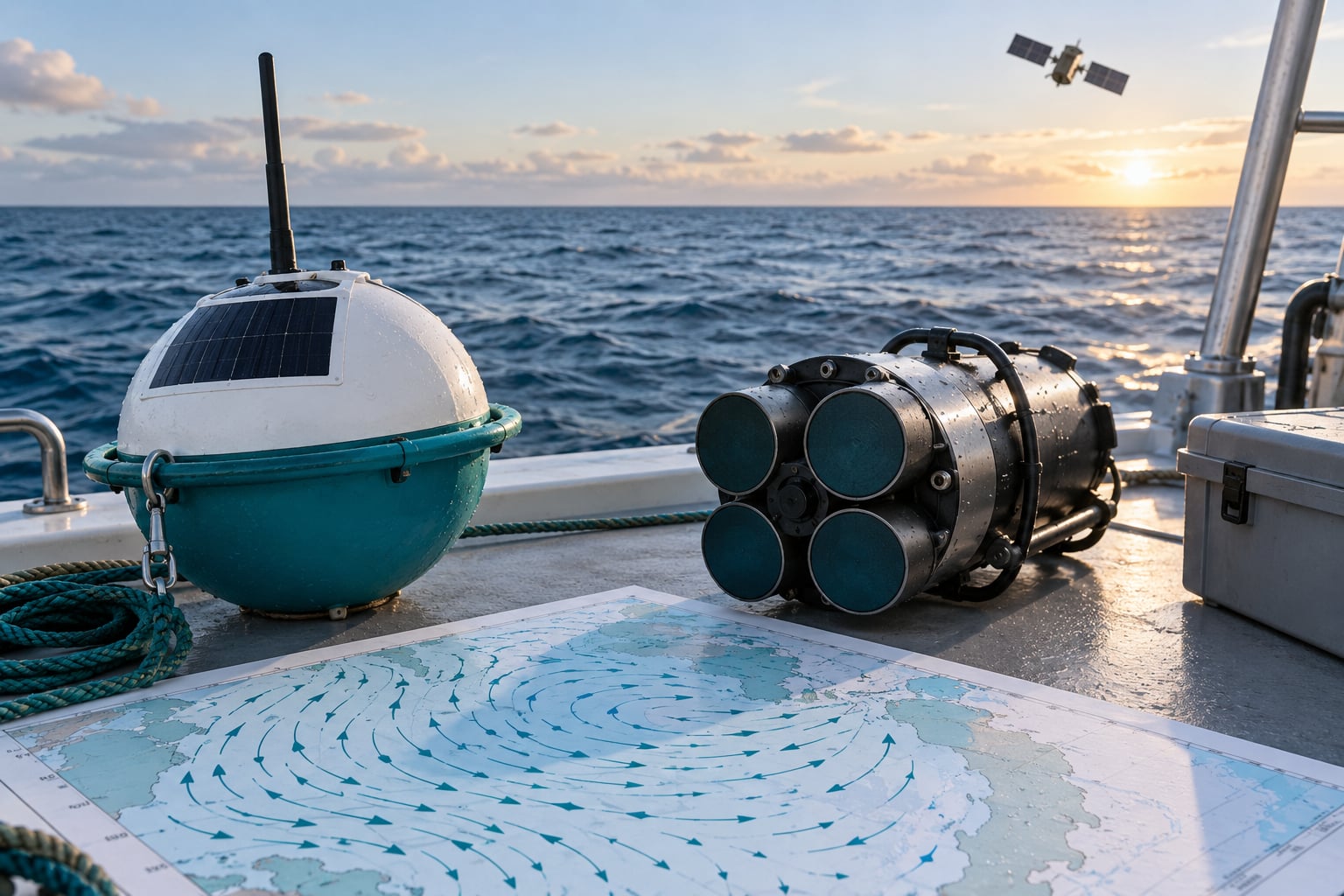
Ocean currents are measured in three broad ways: by following something as it drifts (Lagrangian methods such as surface drifters and Argo floats), by holding an instrument still and watching the water move past it (Eulerian methods such as acoustic Doppler current profilers and moored current meters), or by inferring flow from sea surface height measured by satellite radar (indirect remote sensing). In practice, serious projects mix all three.
Each family answers a different question. A drifter tells you how fast a parcel of water moves and where it ends up. A ship-mounted profiler tells you the speed and direction of every layer beneath the hull, once, to a high precision. A satellite tells you the shape of the surface flow across an entire basin, at a resolution too coarse for a harbour approach.
This guide walks through the instruments in each family, the physics that makes them work, the published limits on their accuracy, and the failure modes that quietly corrupt data. It is written for people who need the numbers rather than for people who need to be impressed by them.
Table of Contents
- What Is an Ocean Current?
- Why Measure Ocean Currents?
- What Do Ocean-Current Measurements Record?
- How Ocean Currents Are Measured: The Main Methods
- How Do Drifting Objects and Surface Current Trackers Work?
- How Do ADCPs Measure Currents Under a Boat?
- How Do Moored Buoys and Fixed Sensors Measure Flow?
- Can Satellites Measure Ocean Currents?
- How Do You Choose a Method for a Boat or Ocean Robot?
- How to Combine Measurements for Better Current Maps
- What Are the Main Measurement Errors?
- Frequently Asked Questions
- Conclusion
What Is an Ocean Current?
An ocean current is a sustained flow of seawater set in motion by wind stress, density differences from heating and salinity, tides, or the Earth’s rotation. It moves slowly and steadily compared with the surface chop, which is exactly why measuring it is harder than it sounds.
Currents are not waves. A wave is an oscillation that travels through the water and returns energy to the surface; the water itself stays roughly in place. A current is a translation: the water is going somewhere. Tides are currents too, but they reverse on a fixed astronomical schedule rather than persisting.
Any current measurement has to resolve four properties: speed, direction, depth, and how much the flow varies over time. An instrument that gives you a single number without saying which depth it applies to is not much use for anything except a headline.
Why Measure Ocean Currents?
Current data decides things with money and safety attached. Offshore wind developers need a year of baseline flow at a site before they fix a foundation position. Harbour engineers need to know how hard water pushes against a breakwater during a storm surge, and how much sediment a channel moves after a dredging campaign.
Environmental work depends on it too. Predicting where an oil spill or a field of floating debris ends up after a storm is a trajectory calculation, and a trajectory calculation runs on measured currents. Sediment transport, aquaculture siting and habitat mapping for shallow reefs or kelp beds all start with the same velocity field.
For researchers, currents carry heat, carbon and nutrients between basins, so the global climate record is written in current measurements. Forecast centres assimilate this data into numerical models, which means every gap in a time series eventually becomes a gap in a weather forecast.
One caution applies to all of it: the surface and the subsurface are different places. A satellite senses the top few centimetres; a current meter at 80 m on a mooring line knows nothing about what the surface is doing. Always match the measurement depth to the question.
What Do Ocean-Current Measurements Record?
Most raw files from a current instrument are small, and most of the fields below are the ones worth checking before you trust a product.
| Quantity | What it means | Typical source |
|---|---|---|
| Velocity | Speed and direction, usually as east/north/up components | ADCP, current meter, drifter, model |
| Depth | Height above the seabed or below the surface | Pressure sensor, known bin spacing, echo sounder |
| Position | Latitude, longitude and time of the fix | GPS or Argos on the drifter |
| Time | Sample interval, from seconds on a ship to hours on a float | All instruments |
| Water level | Sea surface height and its anomaly from a mean | Altimeter, tide gauge, inverted echo sounder |
| Temperature | Water temperature, used with salinity to compute density | CTD on a profiler or float |
| Salinity | Conductivity converted to practical salinity | CTD |
| Bottom pressure | Pressure at the seabed, corrected for the inverted barometer effect | Bottom pressure recorder |
| Transport | Derived: flow through a section, in volume per time | Calculation from velocity across a transect |
| Variability | Derived: tidal currents, eddies, variance, trends | Statistics on the record |
How Ocean Currents Are Measured: The Main Methods
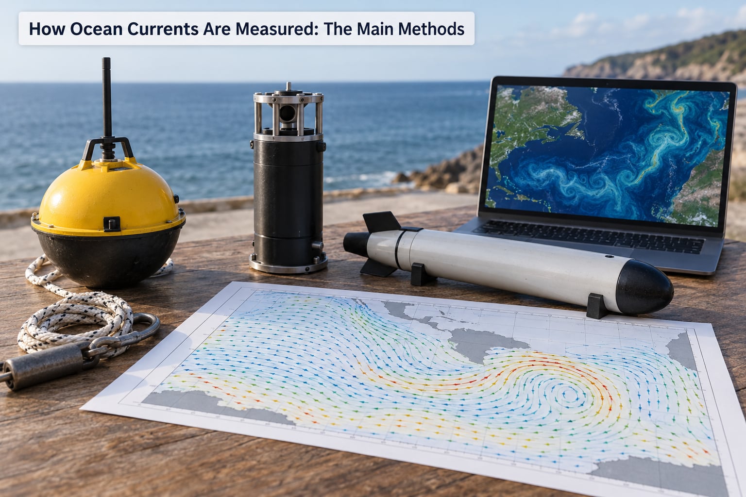
The whole field splits into three families, and the split is about where the instrument sits relative to the water.
- Direct tracking (Lagrangian methods) put an object into the current and record where it goes, giving the path a water parcel actually travelled rather than the flow past a fixed spot.
- Fixed-point instruments (Eulerian methods) stay at one spot or on one line and measure velocity as the water passes, giving a clean time series at a known depth.
- Indirect observation (remote sensing) infers surface velocity from sea surface height or ocean colour, covering whole basins without touching the water.
Under Lagrangian sits the surface drifter and the Argo profiling float. Under Eulerian sit the acoustic Doppler current profiler, the mechanical or electromagnetic current meter, the mooring, and the lowered profiler on a profiling CTD rosette. Under indirect sits radar altimetry, scatterometry, and bottom pressure records from gravity missions.
Advancing one family does not retire the others. Satellites give broad coverage; a mooring gives a century-long series at one point; an ADCP gives detail that nothing else can, for the few hours a vessel is on station.
How Do Drifting Objects and Surface Current Trackers Work?
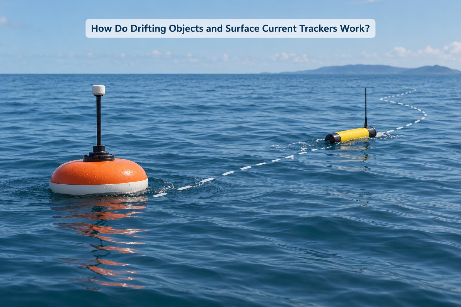
A surface drifter is a drogue plus a hole in the sea surface. The drogue sits well below the surface at a fixed depth and drags the surface float with it, while a GPS receiver and a satellite transmitter on top log position every few hours.
Velocity is then simple arithmetic: the difference between two fixes divided by the time between them. Anything that complicates that arithmetic comes from the mismatch between the drogue and the sensor. Wind pushes on the exposed float, waves drag it forward and back, and shallow-water stiction can stall a drogue near the bottom.
The standard corrections subtract a wind slip term and a wave-induced velocity term, both of which depend on wind speed and wave height. In moderate weather a well-drogued drifter tracks the flow at its drogue depth to within a few centimetres per second. Shallow water is harder, and a drogue touching bottom produces a speed that reads far too low.
Argo floats do the same job at depth. A float adjusts its buoyancy by pumping oil into an external bladder, sinks to a parking depth around 1000 m, rises through a profile measuring temperature and salinity with a CTD, surfaces, transmits by satellite and repeats on roughly a ten-day cycle to about 2000 m. Position change between surfacings gives a velocity averaged over the parking depth.
That averaged velocity is genuinely useful for ocean heat content and deep circulation studies, and it comes with a warning: floats were designed to profile water properties, not to resolve current velocity. The parking depth is set by density, so the float sits wherever it sinks, not at a fixed altitude above the seabed. Treat deep float velocities as a coarse estimate.
Dye releases, drift cards and tracked debris are the older versions of the same idea. They still work in harbours and lagoons where nothing else fits, and they fail in the same place — they tell you about one parcel of water, at one depth, for one period of time.
How Do ADCPs Measure Currents Under a Boat?
An acoustic Doppler current profiler, or ADCP, transmits a sound pulse and listens for the echo scattered back by particles — plankton, sediment, bubbles — that move with the water. The scatterers act like a tiny moving target, and the frequency of the returning echo shifts in proportion to their speed along the beam.
That Doppler shift is the whole measurement. The instrument fires along four beams in a Janus configuration, works out the along-beam component of water velocity for each beam, and combines the four components into a full three-dimensional vector. Because it is time-gated, the returns separate into depth bins, so a single instrument produces a vertical velocity profile rather than a single point.
In bottom-track mode the instrument also measures its own motion over the seabed, which gives an absolute velocity rather than water-relative velocity. Vessel-mounted units run in water-track mode by default, because the ship is not over a fixed seabed reference.
The difficult parts are not the physics. A ship-mounted ADCP sees the hull’s heave, roll, pitch and yaw, and the vessel’s own forward speed pollutes the measurement, so heading, pitch, roll and GPS position must be combined with a precise heading sensor before the data means anything. A common mistake is to leave the tilt correction off and interpret the result in the wrong reference frame entirely.
There are five deployment modes. Vessel-mounted for a survey underway. Lowered, or LADCP, where the unit hangs beneath a CTD rosette on a cable and returns to the ship on winch. Bottom-mounted and upward-looking, recording on a mooring. Towed, trailing behind a boat at survey speed. And moored, climbing a line or a cage at fixed depths.
Each mode has its own blind spot. A vessel-mounted head has a blanking distance, typically a metre or so above the transducers, where it cannot resolve the near-surface flow. A LADCP loses beam data in the first few hundred metres below the head, so the deep shear has to be stitched to the surface head’s bottom track. A bottom-mounted upward-looking unit has the opposite problem, with its weakest zone at the surface.
How Do Moored Buoys and Fixed Sensors Measure Flow?
A mooring holds a sensor at one place for months. The array hangs from a surface float and anchor, with current meters at chosen depths, sometimes a CTD, sometimes an upward-looking ADCP to sample between them, and often an acoustic release to bring the gear back up.
A moored current meter is usually either mechanical — a propeller or rotor turning in the flow — or acoustic, measuring the Doppler shift from a fixed beam. Acoustic meters hold their calibration better in biofouled water and give a direction as well as a speed; rotor meters are simple, cheap and readable, and can drift in calibration after fouling.
Power and logging are the real constraints. A surface buoy can carry solar panels, which lets it run for a year or more. A subsurface node below the thermocline runs on a battery sized for the deployment, and the battery is usually what decides how long the deployment lasts. Data goes out acoustically to the surface buoy and on by satellite, or waits on an internal logger until recovery.
Recovery planning matters more than most people expect. Mooring swing at the surface is a big source of error in measured speed, because the mooring is itself moving through the water and the sensor cannot tell the difference. A common fix is to run an independent measure of mooring motion, often a second acoustic sensor on the line, and subtract it from the flow record. Biofouling on a sensor left for months slowly changes the calibration unless it is checked against a reference.
Can Satellites Measure Ocean Currents?
Yes, but only the surface layer. A radar altimeter measures sea surface height to a couple of centimetres by timing how long a microwave pulse takes to bounce off the sea, and a grid of those measurements across an ocean lets you work out where the water is flowing.
The step that surprises people is what happens between height and velocity. Surface height is sloped by the Earth’s rotation: the Coriolis force pushes moving water to the right in the northern hemisphere and to the left in the southern one, until the slope balances the push. That balance is the geostrophic assumption, and once you have it, a slope in sea surface height converts directly into a current vector through depth-averaged flow.
In short: a hill in sea surface height means water is being steered to one side, and the size of the tilt tells you how fast. The result is a surface geostrophic current, typically with the top few hundred metres represented in the average. It does not resolve the deep flow, and near a coast or in a narrow strait where the water is shallow and the rotation has less room to act, the assumption weakens badly.
Scatterometers measure wind speed and direction over the surface, which combine with the geostrophic relation to give a surface current directly. Optical and microwave imagery can find fronts, eddies and slicks, and thermal and microwave sensors map sea surface temperature and salinity. The Surface Water and Ocean Topography mission adds a fine-swath height measurement that resolves much smaller features than earlier nadir-looking altimeters could.
Satellites are validated against in-situ data constantly. An altimeter that says the Gulf Stream is at a certain position is checked against moorings, drifters and ship transects, and the comparison is part of the mission’s science. Treat satellite currents as a well-supported regional picture rather than a survey-grade local measurement.
How Do You Choose a Method for a Boat or Ocean Robot?
Start from the question, not the instrument. Are you mapping a pattern across an area, holding one point over a season, or profiling layers during a single pass? Each of those wants a different tool, and the cheapest answer is usually the one that matches the shape of the problem.
| Method | Depth range | Endurance | Real-time data | Deployment | Relative cost |
|---|---|---|---|---|---|
| Surface drifter | Surface to a few hundred m | Months | Yes, via satellite | Hand deployed | Low |
| Argo float | Surface to 2000 m, 4000 m for deep variants | 3 to 5 years | Yes, at the surface | Ship-deployed, sea-recovered | Moderate |
| Vessel-mounted ADCP | Blanking distance to a few hundred m | Days of survey time | Yes, live | Needs a vessel with a clean, level flow path | High |
| Lowered ADCP | Surface to full water column | Station time | No, after recovery | Winch, CTD rosette, dive team | High |
| Moored current meter | Any depth in the moored range | Months to a year | Sometimes, via surface buoy | Ship, crane, recovery required | Moderate |
| Bottom-mounted ADCP | Seabed to a few hundred m up | Months on a battery | Sometimes, acoustic to buoy | Underwater deployment | Moderate |
| Satellite altimetry | Surface only | Continuous | Yes, days to weeks later | None, passive | Free public data |
| Build-your-own drifter or logger | Surface only | Limited by power budget | Sometimes | Hand deployed | Very low |
For a small boat with no large vessel and no dive team, the choice narrows fast. A hull-mounted ADCP needs a clean flow path and enough depth beneath the keel; in shallow water, around a few metres, you are mostly limited by the blanking distance and side-lobe contamination near the surface. Field comparisons between low-power Doppler sensor platforms and a conventional workhorse ADCP over multi-week deployments have produced nearly identical speed and direction records, from something two people can put in the water by hand.
For an ocean robot, the binding constraints are power and depth rating. Acoustic profiling drains a battery fast, so most autonomous surface vehicles sample on a schedule and accept a gap between profiles rather than running continuously. If the vehicle cannot log anywhere near the vehicle’s own speed relative to the water, a cheaper mechanical option can be the more honest one.
Ask two more questions. Do you need the data during the deployment, which rules out anything that stores data until recovery? And can you independently validate what you measure, which usually means choosing a method with a public counterpart dataset.
How to Combine Measurements for Better Current Maps
No single method covers both scale and detail, which is why current fields are almost always assembled from several. Satellites give broad coverage and catch the mesoscale eddies; moorings give the long, continuous record at a few points; ADCP transects give the cross-section structure; drifters give the path of individual parcels. Numerical models then fill the gaps between observations and provide the dynamics that explain what was seen.
The usual workflow starts with a satellite map as the background field, then overlays the in-situ data and lets the observations correct the model where they disagree. Modern systems do this by data assimilation: the model is run forward, the observations are ingested with their error bars, and the analysis ends up as the best compromise between the model and the measurements.
Uncertainty should travel with the result, not get quietly dropped. Every derived field inherits the error of the measurements behind it plus the error of the model interpolation, and the two are not independent. Reporting a current map without an uncertainty range is a choice, even if nobody says so.
Free public data makes this genuinely testable without buying anything. Argo profiles and float trajectories, NOAA coastal and oceanic data, and global drifter records cover most of the world’s ocean. A small boat project can pull a nearby drifter track or a float profile and ask whether its own measurements are consistent with the published field.
What Are the Main Measurement Errors?
Most bad current data is not broken data. It is good data with one systematic problem that nobody checked.
| Error source | What it does to the data | Practical mitigation |
|---|---|---|
| Near-surface side lobes | Spurious near-surface velocities above the blanking distance | Discard the top bins, or model the surface layer separately |
| Bubbles and plankton | Contaminated backscatter, wrong or missing bins | Good backscatter screening and bin rejection |
| Vessel motion and tilt | Heave and roll contaminate the velocity vector | High-rate attitude data and a precise heading sensor |
| Wrong reference frame | Spurious vectors when instrument, GPS and model frames differ | Fix the frame once, in the processing, and document it |
| Mooring swing | Sensor motion counted as water flow | Measure mooring motion independently and subtract it |
| Biofouling | Slow drift in calibration over months | Pre- and post-deployment calibration checks |
| Drifter wind slip | Surface float driven faster than the water | Drogue at depth; apply wind and wave corrections |
| Shallow-water stiction | Drogue drags on the seabed, speed reads far too low | Keep drogue depth clear of the bottom; check the record |
| Changing depth | Records at different depths compared as if equal | Log pressure at every sample and bin by depth |
| Sparse sampling | Short record read as a long-term mean | Report the sampling rate and the record length with the number |
| Model assumptions | Geostrophic estimate fails in shallow or narrow water | Use in-situ measurements to test the assumption locally |
| Unit and sign errors | Depth offsets, degrees vs radians, sign conventions | Convert once, in one documented script |
On the CROCO ocean modelling forum, practitioners regularly run into unrealistically high current magnitudes after a configuration change, and the useful part of those threads is always the same: check the reference frames and the units before you change the physics.
Frequently Asked Questions
How does an ADCP work?
An acoustic Doppler current profiler transmits a sound pulse and listens for the echo scattered back by particles moving with the water, such as plankton or sediment. That echo is Doppler-shifted in proportion to the particle speed along the beam. The instrument fires along four beams, converts each frequency shift into a velocity component, and combines them into a three-dimensional vector. Because the returns are time-gated, each ping resolves a range bin, producing a vertical velocity profile instead of a single point.
What do ADCPs measure?
An ADCP measures the speed and direction of water motion as a function of depth, plus acoustic backscatter strength, which indicates how much scatterer material sits in each bin. Most units return three velocity components per bin. They do not measure temperature or salinity; those come from a separate CTD, usually mounted alongside. Instruments configured for bottom track also measure their own motion over the seabed, which is what converts a water-relative velocity into an absolute one.
How accurate are ADCP measurements?
A well-calibrated ADCP measuring clean velocity components typically holds a few millimetres per second, and often far better. Real-world accuracy is limited by the environment, not the instrument: the top bins near the blanking distance, bubble-rich or biologically productive water, strong turbulence, and vessel motion all push the error up. Practitioner experience is that moored swing and uncorrected attitude are the two errors that most often dominate a record, and both are correctable in post-processing if the supporting data were logged.
What is the difference between Lagrangian and Eulerian measurement?
A Lagrangian measurement follows a moving object: a drifter, an Argo float, a drift card. It tells you the actual path a water parcel took over time, which suits transport questions and naturally averages over space. An Eulerian measurement stays at one spot and measures water flowing past, giving a fast, high-resolution time series at a known depth. Neither is better. The choice depends on whether you need the path of a parcel or the flow at a fixed point.
Can ocean currents be measured from space?
Satellites measure sea surface height to a couple of centimetres using radar altimetry, and a slope in that height field converts into a surface current through the geostrophic assumption, where the Coriolis force balances the pressure gradient. That gives a depth-averaged surface current across whole basins, free of charge and continuously updated. It does not see the deep flow, and it weakens in shallow or narrow water where the assumption breaks down, so in-situ instruments are still needed to validate and to measure subsurface conditions.
What is a moored current meter?
A moored current meter is an instrument attached to a mooring line at a chosen depth, recording speed and direction where it sits for weeks or months. Units are either mechanical, using a rotor or propeller, or acoustic, using the Doppler shift from a fixed beam. Acoustic meters resist biofouling drift better and return direction directly. The main limitation is that the sensor only knows its own point, and mooring swing can add a false flow signal unless mooring motion is measured independently.
Conclusion
How ocean currents are measured comes down to where the instrument sits: follow something as it drifts, fix an instrument and watch the water move past it, or infer surface flow from sea surface height. Almost every serious picture of an ocean current combines those three, because each one is blind to something the others see.
If you are starting a project, define the depth range and the accuracy you actually need first, then pick a method that matches. If you can get in the water, calibrate before and after the deployment, log depth and attitude with every sample, and compare the result against a public dataset such as an Argo profile or a drifter track.
Last reviewed: October 2026. Altimetry missions, the Argo array and instrument capabilities all move on, so check the current mission documentation before you commit to a design.