How to Clean Messy Field Data: Workflow for Sensors 2026

Messy field data is any sensor or deployment log that got degraded between collection and analysis, usually by biofouling, sensor drift, spikes, clock drift, saturation or comms dropouts rather than by typing errors. To clean messy field data you work in ordered passes on a copy, never on the original: preserve, inventory, fix time and measurements, deduplicate, then decide for every anomaly whether it is an instrument error or real signal.

A month of one-minute data from a single buoy logger takes an hour or two to clean properly. The payoff is a dataset that survives a second person’s review six months later, when the hardware is in a drawer and nobody remembers what happened on day nine.

The order of operations matters more than the tools. Fix timestamps before you compare neighbours, declare measurement units before you plot, and never delete anything you cannot explain in a sentence.

Table of Contents

• What You Need
• Step-by-Step: How to Clean Messy Field Data Without Losing the Signal
  • 1. Preserve the Raw Data and Create a Working Copy
  • 2. Inventory Files, Rows, Columns, and Field Notes
  • How to Clean Messy Field Data in a Reusable Copy
  • 4. Fix Timezones, Timestamps, and Sampling Order
  • 5. Standardize Measurements, Types, and Identifiers
  • 6. Remove Duplicates and Resolve Missing or Invalid Values
• Visual Example: Raw and Cleaned Sensor Traces
• Common Mistakes That Ruin Field Datasets
• Frequently Asked Questions
  • Should missing field data be deleted or interpolated?
  • How can I tell whether a sensor outlier is real or erroneous?
  • Is it safe to correct timestamps after a deployment?
  • Should I use CSV or Parquet for cleaned sensor data?
  • How should multiple deployment files and calibration records be combined?
• Conclusion

What You Need

Before touching a single value, gather these eight things. Missing any one of them turns a cleanup into guesswork.

• An untouched copy of every raw file. Checksummed, read-only, stored somewhere the analysis script cannot reach.
• A data dictionary. One row per column: name, meaning, measurement unit, valid range, sensor model, calibration date.
• Field notes. Deployment log, recovery notes, weather observations, anything written while wet and cold.
• Source timestamp information. Timezone, clock source, whether the logger drifts, and any known clock resets.
• Declared measurement units per column. The source unit and the target unit, written down before conversion.
• Validation rules tied to physical limits. Sensor range, plausible rate of change, maximum plausible gap.
• Version control or a change log. Git, DVC, or at minimum a dated text file listing every rule you applied.
• Analysis software. The examples below use Python 3.12 with pandas 2.x; a spreadsheet can do the same operations, more slowly.

If you cannot get a data dictionary, build one from the logger’s configuration file and the calibration record. That is most of the work anyway.

Step-by-Step: How to Clean Messy Field Data Without Losing the Signal

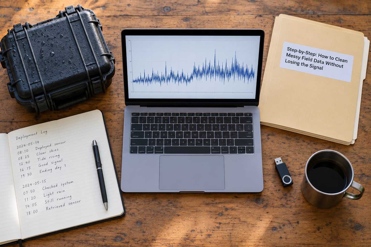
The workflow has seven stages. Every transformation should be repeatable, reviewable, and applied to a working copy rather than to the original field files. Step three has a longer heading than the others because it is the stage people search for by name.

1. Preserve the Raw Data and Create a Working Copy

Hash every raw file, then make the raw directory read-only. On Linux or macOS that is chmod -R a-w raw/, and the hash command is sha256sum on Linux, shasum -a 256 on macOS.

Write the hashes into a manifest file next to the data. If a cleaning script ever touches a raw file by accident, the hash mismatch tells you immediately rather than six months later.

Then copy raw into a working folder and do all editing there. Record the software versions you used, because a cleanup that depends on library behaviour is not reproducible if nobody knows which library was installed.

# raw/ stays read-only; every script reads from raw/ and writes to work/
df = pd.read_csv("raw/dep_041.csv", parse_dates=["log_time_local"])
df.to_parquet("work/dep_041_stage0.parquet", index=False)
open("work/manifest.txt", "a").write(f"pandas {pd.__version__}npython {sys.version}n")

You should be able to rebuild every downstream file from raw/ plus one script. If you cannot, the cleanup was manual work, and manual work on field data is where mistakes get frozen in.

2. Inventory Files, Rows, Columns, and Field Notes

Build an inventory before you build anything else: file name, sensor, measurement unit, sampling rate, first and last timestamp, deployment ID, known interruptions, and files you are missing. A deployment that shipped with a firmware bug often produces a truncated file nobody mentioned, and you find it here rather than three steps later.

Then link the log to everything else you have. Mission notes tell you when the vehicle surfaced and transmitted; calibration records tell you when a sensor was last checked; weather observations explain temperature swings; robot status events explain power loss.

This is where field data stops being an abstraction. Two files with the same column names, the same deployment ID and a one-hour overlap usually mean a re-deployed logger with a fresh config, not a duplicated file.

Profile the numbers while you are there. Per column: row count, null count, minimum, maximum, and the modal gap between consecutive timestamps. A modal interval of exactly 60.0 seconds tells you the intended sampling rate, which every later check depends on.

gap = df["log_time_local"].diff().dt.total_seconds()
profile = {
    "rows": len(df),
    "nulls": df.isna().sum().to_dict(),
    "min": df.select_dtypes("number").min().to_dict(),
    "max": df.select_dtypes("number").max().to_dict(),
    "modal_gap_s": gap.mode().iat[0],
    "max_gap_s": gap.max(),
}

How to Clean Messy Field Data in a Reusable Copy

The working copy needs four things standardised before values are touched: file handling, column names, missing-value encoding, and identifiers. Do it in code so the same pass runs on tomorrow’s file.

File handling means one schema per deployment: same column order, same separators, same encoding, same timestamp format. Column names go to a consistent case and vocabulary, so Temp, TEMP_C and temp (C) all become temp_c.

Missing values get one encoding everywhere. Pick NaN for “no measurement exists” and a separate sentinel such as -999 for “the sensor reported a fault code”, because those two cases deserve different treatment downstream.

Identifiers get their own pass. Deployment ID, sensor serial, file name and a per-row record ID should be unique and non-null before you merge anything. Conflicting deployment identifiers are the single fastest way to build a dataset where two different sites overlap for six hours.

RENAME = {"Temp": "temp_c", "TEMP_C": "temp_c", "temp (C)": "temp_c"}
SENTINELS = {"temp_c": [-999, 9999]}

df = (df.rename(columns=lambda c: RENAME.get(c, c.strip().lower()))
        .replace(SENTINELS, other=pd.NA)
        .sort_values(["deployment_id", "time_utc"])
        .drop_duplicates(subset=["deployment_id", "time_utc"], keep="first"))
assert df["deployment_id"].notna().all()
df.to_parquet("work/dep_041_stage1.parquet", index=False)

Keep the original columns alongside the cleaned ones. Six months on, the question “was this 12.4 metres or 1.24 bar?” gets answered in seconds instead of by guesswork.

4. Fix Timezones, Timestamps, and Sampling Order

Field data fails at the clock more often than people expect. Loggers record local time, boats cross timezones, deployments sit in daylight-saving transitions, and cheap boards drift by seconds per day until the log is a plausible but wrong timeline.

Convert to UTC at the start and keep UTC everywhere after that. Sorting before conversion hides the problem instead of fixing it.

df["time_utc"] = pd.to_datetime(df["log_time_local"], utc=True, format="mixed")
df = df.sort_values("time_utc").reset_index(drop=True)
dups = df["time_utc"].duplicated().sum()
nonmono = int((df["time_utc"].diff().dt.total_seconds() < 0).sum())

Two error types need different handling. Duplicate timestamps from a logger that writes twice on retry are exact duplicates, and you keep the first. A non-monotonic timestamp usually means a clock reset, and correcting it requires evidence: a transmission event in the mission log, a surface GPS fix, a known power cycle.

Clock drift is the quiet one. Compare the logger clock against a reference you trust, plot the difference against time, and if the slope is steady you have a linear drift term you can apply. If the difference jumps, you have a reset, and you correct each segment separately.

Never overwrite a timestamp silently. Add a time_correction_s column and a time_confidence value of high, medium or low. A corrected timestamp with a stated confidence is a result; a corrected timestamp with no note is a rumour.

Finally, do not assume equal sampling. Compute the real interval distribution and check it against the configured rate. Sensors that buffer and burst-report produce a dataset with a modal gap of zero and a long tail, which breaks any filter that assumes a fixed window.

5. Standardize Measurements, Types, and Identifiers

Declare one unit per column and convert to it explicitly. Temperature, pressure, depth, speed, heading, conductivity: each one gets a named source unit, a named target unit, and a conversion you can see in the script.

Depth is the usual trap. A pressure sensor in millibars, a depth sensor in metres, and a pressure-derived depth in metres are three different columns wearing the same name. Convert one explicitly, keep the source column, and record which sensor produced which value.

df["depth_m"] = df["pressure_dbar"] / 1.0        # 1 dbar of seawater ~ 1 m
df["temp_c"] = (df["temp_f"] - 32) * 5 / 9         # only if the source really is Fahrenheit
df["heading_deg"] = df["heading_deg"] % 360        # wrap, do not renumber
for col in ["temp_c", "depth_m", "heading_deg"]:
    df[col] = pd.to_numeric(df[col], errors="coerce")

Enforce types next. Numeric columns become numeric, category columns become a fixed set of allowed labels, and anything that fails conversion goes to missing with a flag rather than silently becoming zero. Casing variants, trailing spaces and abbreviated names in categorical fields are a schema problem, not a data problem, so fix them in the naming pass.

Heading deserves one more note. A magnetic compass heading near 0 and 360 degrees is the same bearing split across the wrap, so treat the column as circular when you average or filter it.

6. Remove Duplicates and Resolve Missing or Invalid Values

Start by separating exact duplicates from valid repeated readings. A repeated timestamp with identical values is a logging artefact. Two identical values a minute apart from a slow sensor are the signal.

Then classify every anomaly against physical limits rather than against statistical comfort. Sensor range, plausible rate of change, and the deployment context tell you more than any z-score. Before you delete anything, work through this list of field failure modes.

• Single-sample spike. One value far outside its neighbours, returning immediately. Symptom: a single reading 15 standard deviations out. Detection: a rolling median filter or a Hampel filter, which uses the median absolute deviation instead of the standard deviation so one spike cannot inflate its own threshold. Treatment: flag as suspect, replace with the rolling median, keep the original in a separate column. Never delete the row.
• Fouling step change. A slow offset that appears over hours and never recovers. Symptom: biofilms or growth on the sensing surface. Detection: a change-point test, or a long rolling median difference against the pre-deployment baseline. Treatment: apply a documented offset correction or quarantine the period, and label it as fouling rather than a data error.
• Sensor drift. A gradual ramp in the whole record. Detection: a fitted slope against a reference series. Treatment: recalibration offset, or a flag if you have no reference.
• Saturation and clipping. A value pinned at the sensor limit. Detection: runs of identical values at the range boundary. Treatment: flag as out of range, never interpolate across it.
• Power or comms dropout. A contiguous block of missing rows. Detection: a gap far beyond the modal interval, corroborated by a power or transmission event. Treatment: leave the gap empty and flag it, because the gap is a measurement of the platform.
• Unit mismatch. A value plausible for one column and impossible for another. Detection: range checks per unit. Treatment: convert explicitly and keep the source column.

Spikes and step changes are not the same thing. A spike is one sample that disagrees with its own history; a step change is a permanent shift that everything after it agrees with. Despiking filters handle the first, and they will happily flatten a real transition if you let them.

A Hampel filter is the workhorse for sensor traces. It compares each sample to the rolling median and flags anything beyond a scaled median absolute deviation, which makes it resistant to the very spikes it is looking for.

def hampel_flags(series, window=11, n_sigma=3.0):
    med = series.rolling(window, center=True, min_periods=1).median()
    dev = (series - med).abs()
    mad = dev.rolling(window, center=True, min_periods=1).median()
    scale = 1.4826 * mad
    scale = scale.where(scale > 1e-9, other=series.abs().median() * 1e-3)
    return dev > n_sigma * scale

df["qc_temp"] = np.where(hampel_flags(df["temp_c"]), "suspect_spike", "good")
df["temp_c_clean"] = df["temp_c"].where(df["qc_temp"] == "good")
df["temp_c_clean"] = df["temp_c_clean"].rolling(11, center=True, min_periods=1).median()
df["temp_c_raw"] = df["temp_c"]

On gaps, the rule is simple: interpolate only short gaps between valid samples, and only when the variable is physically smooth over that window. A temperature probe can carry a 30-second gap. A power state cannot carry anything. Long gaps and any gap in a state or event column stay empty.

Do not fill systematic gaps at all. Gaps caused by power, biofouling or radio loss are not missing at random, and averaging over them quietly fabricates conditions that never happened.

Impute only when the analysis demands a complete series, and record how many values you inserted. A published result with an undisclosed fill is a result nobody can defend.

Visual Example: Raw and Cleaned Sensor Traces

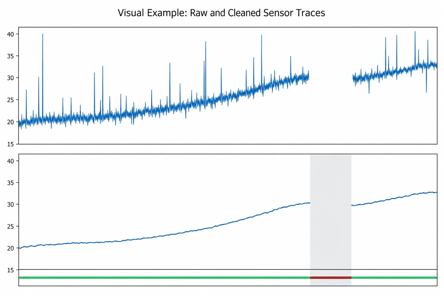
One before-and-after plot tells you whether the cleanup worked. Plot the raw trace and the cleaned trace on the same axes, with the gap shaded rather than interpolated, and a thin channel underneath showing the quality flag for each sample.

Read the cleaned panel critically. If the tidal structure survives, the fouling step is still visible as a slow offset, and the gap is still a gap, the pipeline did its job. If the cleaned trace is smooth and featureless, you have removed the signal along with the noise, and the despiking window is too wide or the threshold too aggressive.

Keep these plots in the repository next to the data. They are the fastest defence you have when someone asks why a value was changed, and the fastest way to spot a cleanup step that went wrong months later.

Common Mistakes That Ruin Field Datasets

Overwriting the raw file. The fix is boring and absolute: read-only originals, hashes, and a manifest. A corrupted raw file with no backup ends the deployment’s usefulness.

Deleting every outlier. Most exciting events in a field record are outliers. The fix is to classify first, then treat: flag and preserve, correct only the values you can defend, and quarantine rather than remove.

Assuming equal sampling. A filter with a fixed window assumes a fixed interval, and buffered loggers break that assumption. The fix is to compute the real interval distribution and index by time rather than by row number.

Changing a unit without writing it down. Depth in millibars versus metres changes a tide chart into nonsense that still looks plausible. The fix is a declared unit per column plus a retained source column.

Interpolating long gaps. A six-hour fill through a power dropout invents six hours of ocean. The fix is to leave the gap empty, flag it, and let the analysis handle missingness honestly.

Mixing deployment identifiers. Two deployments with overlapping timestamps silently become one record. The fix is a composite key of deployment ID and timestamp, checked for uniqueness before anything else runs.

Cleaning with no record of what changed. If nobody can say which rules ran, the dataset cannot be re-processed when a better filter appears. The fix is a change log with rules, thresholds, software versions, exclusions and flag counts.

Three habits keep this manageable. Version the cleaned dataset alongside the script that produced it. Keep the data dictionary in the same repository, updated in the same commit. And have a second person review the before-and-after plots before the data leaves the team; almost every catastrophic cleaning error is obvious in a plot and invisible in a row count.

Frequently Asked Questions

Conclusion

To clean messy field data, run seven passes in a fixed order: preserve, inventory, standardise, fix time, fix measurements, classify anomalies, validate and document. The raw files stay untouched, every anomaly is labelled as instrument error or real signal, and every decision is written down.

Start with the first step today rather than the fifth. Checksum the raw files, make them read-only, and write down what you already know about deployment interruptions, calibration dates and sensor problems, while the field notes are still in your head.