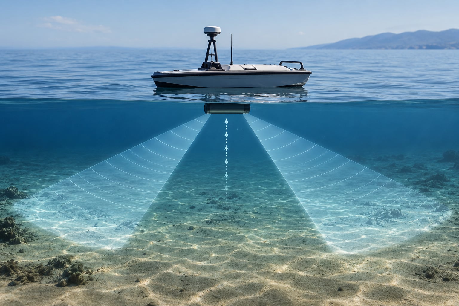
Side scan sonar sends a short acoustic pulse sideways, to port and starboard, then listens for the echo coming back from the seafloor. It measures how long that echo took to return and how strong it was, and turns both numbers into brightness. Understanding how side scan sonar works comes down to those two measurements, and what you get is a two-dimensional picture of the bottom out to each side, built up as the vehicle moves.
That is the whole idea, but the interesting part for anyone building a boat, an AUV or a small robot is what happens between the ping and the pixel. Water is a good carrier for sound and a poor one for light, so a side scan system trades direct depth measurement for enormous coverage, and the picture it produces is geometrically distorted until you correct for it.
Table of Contents
- How Side Scan Sonar Works
- What Side Scan Sonar Measures
- How the Equipment Is Built
- How an Echo Becomes a Sonar Image
- Why Seafloor Features Cast Shadows
- How Sonar Frequency Changes the Map
- How Side Scan Sonar Is Used on Boats and Robots
- What Determines Image Quality
- What Side Scan Sonar Cannot Tell You
- Safety and Survey Best Practices
- Frequently Asked Questions
- Conclusion
How Side Scan Sonar Works
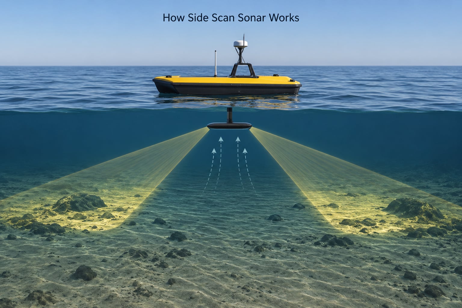
A side scan sonar is an active sonar system. It transmits a brief pulse of sound to both sides, records the intensity and arrival time of the echoes, and stitches those echo records together along the vehicle’s track into a sonogram. Brightness on that image is echo strength, which is why the image reads as texture and shadows rather than as a depth chart.
The signal chain is four steps, and everything else on the page is detail hanging off one of them.
1. Transmit. A piezoelectric transducer is driven by a high-voltage pulse and converts it into a pressure wave in the water. The pulse is short, typically a fraction of a millisecond to a few milliseconds, and narrow in azimuth but wide in elevation, so it fans out across the bottom like light from a desk lamp lying on its side.
2. Receive. The same transducer switches to listening. Every scatterer in the beam sends back a small fraction of the energy, and the arrival time encodes range while the amplitude encodes how hard the target reflects. The receiver amplifies and digitises the return, and a timing system samples it into range bins.
3. Form the image. Each ping produces one narrow strip, or cross-track slice, running from the nadir line outward on each side. The strips are corrected for slant range, scan converted into a rectangular display, and stacked as the vehicle advances, so along-track position comes from motion and across-track position comes from time.
4. Interpret. Bright areas are hard, steeply facing surfaces such as rock, wreck plating, boulder edges or a pipeline. Dark areas behind them are acoustic shadows. The operator or the processing software reads the pattern of bright and dark to decide what is down there.
One number makes all of this concrete. Sound in seawater travels at roughly 1500 metres per second, so range is just half of travel time multiplied by that speed. A return that arrives 4 milliseconds late sits about 3 metres away horizontally, whatever its brightness.
What Side Scan Sonar Measures
Two things, really: how long the echo took to come back, and how much of the transmitted energy it carried. Everything else on the screen is derived from those two measurements.
Two-way travel time is the raw range measurement. The pulse travels out and the echo travels back, so the slant range equals the sound speed times the elapsed time divided by two. A one-millisecond round trip covers about 0.75 metres of water.
Slant range is the distance along that path, which is not the same as the distance across the seabed. A point directly under the fish is at slant range equal to the altitude; a point far out to the side is at a slant range longer than its ground range. This is the source of most of the “the range scale is lying to me” complaints, and slant-range correction deals with it later.
Acoustic intensity, usually logged as backscatter strength, is the amplitude of the return. It scales with the size of the target, its orientation to the beam, the grazing angle, the transmit level, the range, and the reflection coefficient, which in turn depends on the acoustic impedance difference between the target and the surrounding water.
That last point is worth dwelling on. A steel hull sitting in water is a large impedance contrast and returns a lot. Wet sand and soft mud are close to a weak reflector and return little. The sound is not measuring colour or chemistry; it is measuring how badly sound is reflected at an interface.
So brightness is a real signal, but it is a mixed one. The same rock can look bright or dull depending on the sun angle, the water conditions, the sonar gain setting, and the heading of the towfish relative to the slope. A hard bottom facing the sonar returns far more energy than the same hard bottom lying flat.
Interpretation therefore depends on context. A bright linear feature with a matching dark band beside it is almost always a raised object. A uniformly bright field with no shadows is usually a flat hard surface. Once you know what changes the return strength, the image stops looking like abstract art.
How the Equipment Is Built
Every side scan system, whether a towfish or a hull-mounted transducer, contains the same chain of parts, even if the packaging looks completely different.
The transducer is the heart. On professional systems it is a long line array of piezoelectric elements running parallel to the vehicle’s keel, often with separate arrays for port and starboard. On small systems it may be a single wide element, which is why small units usually have a broader, blurrier beam.
Behind it sit a signal generator that produces the transmit pulse, a pulse amplifier that raises it to the hundreds of volts needed to put real energy into water, and a transmit-receive switch that protects the sensitive receiver during the transmit window. That switch is a real engineering problem, because the receiver has to survive a pulse orders of magnitude louder than the echo it is trying to hear, and it only has a few milliseconds to get ready.
Then come the receiver and digitiser, which amplify the weak return and sample it, and the timing and triggering system, which decides when each ping fires and how each return is divided into range bins. Navigation sensors supply position, heading and time, because an image without accurate navigation is just a long smear. Everything finishes in software, which handles gain, slant-range correction, scan conversion and mosaicking.
How Side Scan Sonar Forms a Wide Beam
The beam shape comes from the physical size of the array, the frequency, the acoustic wavelength, and sometimes electronic steering of individual elements. A larger array radiates a narrower beam in azimuth, which concentrates the transmitted energy into a smaller footprint and gives better along-track resolution.
Elevation beamwidth, the vertical part of the fan, is usually deliberately wide, often 20 to 40 degrees, because the geometry of grazing incidence needs to cover from just under the nadir out to maximum range. A narrow elevation beam would leave gaps in the near field.
| Beam behaviour | What causes it | Along-track resolution | Operational tradeoff |
|---|---|---|---|
| Narrow azimuth beam | Long line array, low frequency, wide elements | Fine, detailed streaks along track | Needs a stable mount and steady speed; long range, low ping rate |
| Wide azimuth beam | Short or single-element transducer, high frequency | Coarser, softer along-track detail | Simple, cheap, tolerant of motion, short range, high ping rate |
| Wide elevation beam | Small vertical aperture relative to wavelength | Not applicable | Covers near to far range in one ping, but includes more noise and more multiple returns |
The practical consequence: the same object looks bigger and blurrier the further out it is, because the beam footprint grows with range. Near the nadir line the sonar resolves fine gravel; at the far edge of the swath, a boulder half a metre across is a few pixels of brightness and its shadow is the only clear signal.
Where the transducer lives
A towfish is a torpedo-shaped body streamed behind a vessel on a cable. It stays at a controlled altitude, is usually aerated or depressor-equipped so it flies at depth, and gives the cleanest images because the transducer is well away from hull noise, propellers and bubbles. It also adds layback, a time delay between the fish and the boat’s position that has to be corrected before georeferencing.
A hull mount is cheaper and simpler. The transducer has to sit clear of the hull, or at least see past it, or the shadow of the boat appears in every image. Fixed mounts also move with the hull, so waves change the altitude and the image wobbles.
An ROV or AUV carries the transducer as part of a controlled platform. The vehicle holds altitude with a depth sensor and flies a lawnmower pattern, which makes line spacing and navigation accuracy a software problem. This is where autonomous mapping earns its keep, and where the physics has to be respected rather than assumed.
How an Echo Becomes a Sonar Image
Follow one ping all the way through, and the image stops being magic.
The trigger fires. The pulse leaves the array, the array goes quiet and listens, and the returned energy is sampled at a rate set by the range scale. If the operator selects a 100-metre range per side, the system has 200 metres of water to cover plus the nadir gap, which at 1500 metres per second round trip is about 267 milliseconds of listening time, split into range bins of whatever length gives the desired range resolution.
That bin length sets the range resolution directly. A 100-microsecond pulse length gives roughly 7.5 centimetres of range resolution, because that is how much water the pulse occupies in space. Longer pulses resolve more range but blur along-track detail, because a longer pulse is also a longer transmitted packet of energy that spreads more energy in time.
The raw bins are then slant-range corrected. Ground range is computed from slant range and altitude, so features near the nadir line are not stretched across the display. Without this step, objects at the far edge of the swath are pulled inward and the image geometry is wrong, which is exactly why a wreck looks longer at one range scale than at another.
Scan conversion turns the wedge-shaped slice into a rectangular strip, equalising brightness across the swath so that a distant target is not dimmed purely by spreading loss. Mosaicking overlaps consecutive strips along track, and georeferencing applies position, heading, layback and tide to place the result in map coordinates.
What comes out has two natural axes. Across-track is range. Along-track is time, converted to distance by speed over ground. That is why along-track resolution depends on how fast the vehicle is moving and how often it pings, and why speed instability produces smeared, distorted mosaics.
Motion can also be used rather than fought. Synthetic aperture techniques use the fact that the array is moving to synthesise a much longer effective aperture, then compensate for the movement of each element. It is how fine along-track detail is recovered from sparse samples, and it is why a stable trajectory and a good navigation solution matter so much.
Why Seafloor Features Cast Shadows
A raised object blocks the outgoing pulse, so part of the seabed behind it receives no sound and returns nothing. That unlit strip is the acoustic shadow, and it appears as a dark band trailing away from the nadir line.
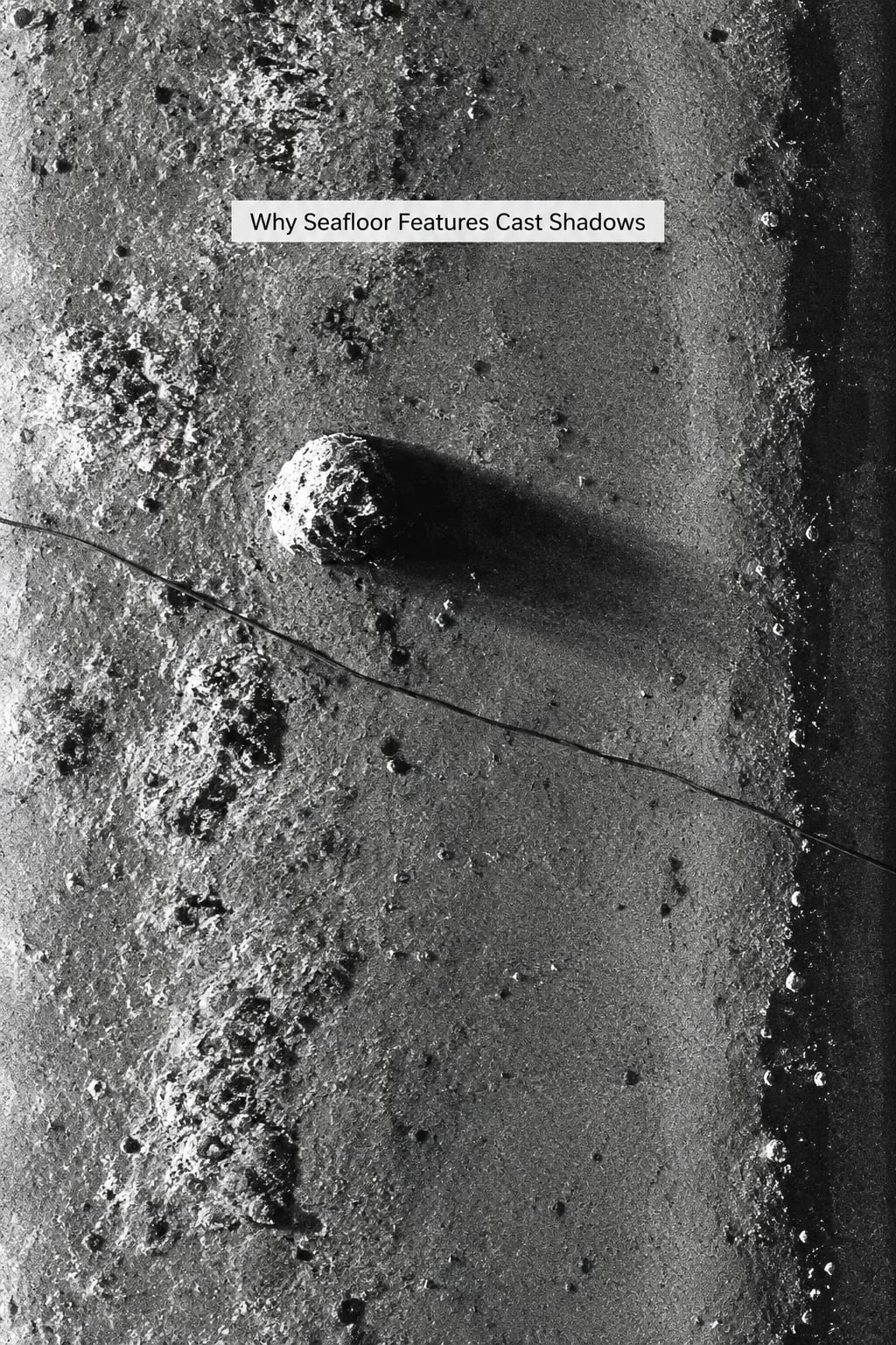
Shadows carry the height information that brightness alone cannot. On a flat, even seabed they should not exist at all, so any shadow means there is something standing proud of the bottom.
The geometry is straightforward. With a towfish altitude a, an object of height h at ground range g, the ray grazing the top of the object continues past it and paints a shadow extending roughly h·g/(a−h) further out. Rearranged, height is about L·a/(g+L) for a measured shadow length L. In practice people estimate it more crudely by eye, and both approaches need a known altitude and a known heading to be worth anything.
Typical signatures are worth memorising. Boulders and rock pinnacles give a compact bright return with a hard-edged shadow whose length tracks height. Wrecks give long bright deck edges, hard returns from superstructure, and shadows that outline a hull shape. Pipelines and cables give a thin continuous bright line with a narrow shadow, and the shadow is often more reliable than the return itself.
Trenches and dredged channels appear as broad dark bands, because the far wall turns away from the sonar and the bottom inside the trench is beyond the grazing geometry that returns well. Sand dunes and ripples show as repeating bright-dark banding whose wavelength is the ripple spacing. Mud and soft sediment return weakly and produce little shadow, which is why a flat, uniform grey field is often simply soft bottom.
None of this is automatic identification. A boulder and a buried mine can look similar, and a debris field and a rock field can look similar. Shadows narrow the possibilities; they do not name the target.
How Sonar Frequency Changes the Map
Frequency sets the wavelength, and the wavelength sets almost everything else. Higher frequency means shorter wavelength, which means smaller scattering features are resolved, which means better texture and finer detail but more attenuation through water and a narrower useful range. Lower frequency pushes further and sees larger, deeper targets but blurs away texture.
Wavelength is just sound speed divided by frequency, so 400 kHz works out around 3.75 millimetres in seawater, and 50 kHz around 30 millimetres.
| Frequency | Approx. wavelength | Typical usable range per side | Best suited to |
|---|---|---|---|
| 50 to 100 kHz | 15 to 30 mm | 300 to 1000 m | Large pipelines, long cable routes, deep penetration, regional mapping |
| 200 kHz | 7.5 mm | 150 to 300 m | General hydrographic survey, seabed mapping, debris fields |
| 400 kHz | 3.75 mm | 75 to 150 m | Wreck surveys, structural detail, dredge and construction clearance |
| 500 kHz | 3 mm | 50 to 100 m | Fine target definition, small debris, ROV and AUV close work |
| CHIRP 540 to 850 kHz | 2.8 to 1.8 mm | 20 to 60 m | Very high resolution small-boat and kayak imaging of structure and fish |
CHIRP is a frequency-swept pulse rather than a single tone. Sweeping from high to low frequency over the pulse length gives much higher bandwidth, so a very short effective pulse and fine range resolution are possible at the same time as lower peak transmit power, which is why it became standard on small boat units.
Beam width is frequency dependent too. A given array is electrically longer at low frequency, so it radiates a narrower azimuth beam; a high-frequency system on the same hull paints a wider, more energetic swath at close range.
Low frequencies are also more exposed to ambient noise. Traffic, wind, rain and vessel machinery all live in the low band, so a 50 kHz channel in a busy harbour can be unusable in a way that 400 kHz is not.
How Side Scan Sonar Is Used on Boats and Robots
Deployment changes everything about the image you get, even when the electronics are identical.
On a survey boat, a towfish is streamed, depressors or aeration are adjusted to hold altitude, and the vessel runs parallel survey lines at a set spacing. Professional operators report that a line spacing of roughly 100 to 200 metres with a 200 kHz system gives good overlap and few gaps; the same rule of thumb is altitude at about 10 to 20 percent of the working range.
On an ROV or AUV, altitude is held by a dedicated sensor rather than by hope, and the vehicle flies a lawnmower pattern with nav fix spacing tight enough to georeference the mosaic. Power draw matters, because the sonar competes with thrusters, lights and computers for the same battery, and pulse repetition rate has to fit inside the loop.
How side scan sonar works on a small autonomous craft
On a small autonomous surface craft, the challenges are different. The hull is short, so the array is short, and the beam is wide. Wave motion moves the transducer up and down relative to the bottom, and the image wobbles; users with small boats report this is motion, not a fault. The fixes are practical: mount the transducer as low as possible, stiffen the mount, damp the electronics housing, run a high ping rate, and accept the extra smearing that comes with each correction.
On a recreational fishfinder, the same physics is packaged as side imaging, usually at CHIRP frequencies, and users report usable ranges of roughly 45 metres per side from a kayak with detail degrading fast at the far edge. Working settings follow a pattern: a narrow range scale, a high-frequency channel, and a colour scheme with strong contrast between hard and soft returns. An experienced charter captain runs 800 kHz on a blue and white scheme at about 24 metres per side, widening to 36 to 45 metres only when hunting schooling forage.
Two operational choices separate a usable survey from a wasted day. Speed sets along-track resolution, since resolution is roughly speed divided by twice the ping rate; going too fast smears targets into streaks. Stopping to collect data is possible but gives up coverage, so continuously pinging while moving is normal even at low speeds.
What Determines Image Quality
Most disappointing side scan imagery comes down to a short list of controllable variables rather than a bad transducer.
Range and altitude set the tradeoff between coverage and detail. Altitude at 10 to 20 percent of the intended range is the usual starting point, and going higher makes everything look stretched and shadow-heavy.
Vehicle speed sets along-track resolution. Small craft in waves vary in speed constantly, and the mosaic inherits that variation as wavy along-track distortion.
Pulse length and bandwidth set range resolution. Shorter pulses resolve finer detail vertically but need more transmit energy to reach the same range.
Sampling rate and range scale set the size of a range bin. A wide range scale on a shallow survey wastes most of the display on empty water.
Water conditions matter more than most people expect. Rough surface, a sandy suspension layer, and thermoclines near the surface all scatter or absorb the signal, and bubbles from wake or from the transducer’s own housing can black out the near field entirely.
Heading stability decides whether shadows point consistently. A towfish that yaws sends shadows sweeping back and forth, which makes feature identification much harder.
Seabed roughness and noise set the contrast you have to work with. A rough sand-and-shell seabed produces a busy image in which small targets hide, and high ambient noise lifts the background so the same gain no longer isolates the target.
A practical first pass, then: pick a range scale slightly wider than the feature you care about, set altitude to a tenth of that range, hold speed steady, set gain so the background sits low and bright features sit near the top of the scale, fly overlapping lines, and log the settings. Then look for the artifacts.
Wavy or shaking images point to motion, not electronics. A hard dark band at a fixed distance that follows the vehicle is usually a surface reflection or a multiple bounce. Bright features that appear at two ranges and move differently are the same object seen directly and again through a reflection. A target that disappears as the vessel turns is a directivity problem, which is what a properly formed beam is supposed to prevent.
What Side Scan Sonar Cannot Tell You
The honest list of blind spots is short, and knowing it prevents most misinterpretation.
It does not give absolute depth under a target. It gives slant range to whatever reflected. To know a target sits at 30 metres rather than 40, you pair side scan with a bathymetric sensor or a depth sensor on the vehicle.
It does not identify material. A bright return might be steel, rock, concrete or a hard gravel patch. Composition needs a calibrated interpretation, sampling, or a different sensor.
It does not see through the seabed. Anything buried has no acoustic contrast until it is exposed, which is what sub-bottom profiling is for.
It does not classify biology. Fish, kelp, a school and a shadow from surface chop can all produce bright returns, and separation often needs polarisation, a water column sensor or a human.
Its shadow-based height estimate degrades with altitude and depends on knowing the towfish height accurately, so it is a good indicator and a poor measurement.
| System | Measures | Typical output | Main limitation |
|---|---|---|---|
| Side scan sonar | Backscatter intensity and time across a wide swath | Sonogram and georeferenced mosaic | No direct depth, distorted geometry, shadows instead of elevation |
| Multibeam echosounder | Travel time across many narrow beams | Depth surface for bathymetry | Higher power, more processing, less backscatter detail than side scan |
| Sub-bottom profiler | Return strength versus time through sediment layers | Stratigraphic section beneath the bottom | Low lateral resolution, needs shallow penetration and calm conditions |
| Optical imaging | Reflected light | Photo or video | Ranges of metres only, fails in turbid water |
In practice these are complements. Multibeam supplies the depth, side scan supplies the texture and the shadows, a sub-bottom profiler supplies the layering, and a camera or ROV video confirms anything that matters operationally.
Safety and Survey Best Practices
Side scan sonar is low power compared with a hull-mounted multibeam, but it is not silent, and it transmits on frequencies that marine mammals use.
Watch for marine life and slow down or stop in areas with visible aggregation, and follow the local rules that apply to your water, since acoustic-source restrictions vary by port, state and country. Avoid operating in the same frequency band close to active navigation or fisheries systems you have not checked with.
Plan around weather rather than around it. Surface conditions set the noise floor and the motion, and both degrade the image. Check the forecast, keep enough sea room for the tow cable, and know the tension limits of the cable you are streaming.
Cable handling is the part that hurts people. A towfish that snags puts sudden load on the winch, so keep hands clear of the drum and the block, and never wrap the line around anything you are holding.
For autonomous work, define the fail-safe behaviour before the mission, not during it. Loss of navigation, loss of altitude control, or a battery state that will not finish the survey should each have a defined, tested response, normally return-to-launch rather than continue-and-deteriorate.
Keep the raw data and the field notes. Raw channels, navigation logs, the altitude record, the settings for every line, and the weather are what let someone re-interpret a survey months later. Processed mosaics alone cannot be reprocessed with a better slant-range model or a different gain.
Frequently Asked Questions
Does side scan sonar measure water depth?
No. Side scan sonar measures the two-way travel time and strength of echoes returning from a wide swath to each side, so it gives slant range to whatever reflected, not the depth of that object. To turn slant range into ground range and know an actual depth, you pair it with a depth sensor on the vehicle or a bathymetric sonar. Without that pairing, features are located in image geometry, and a far-off target at a similar range is hard to separate from a nearby one lying flat.
Can side scan sonar identify the size and material of an object?
It can suggest size and hint at material, but it cannot confirm either. Object height is estimated from the length of the acoustic shadow behind it, and that estimate gets worse as towfish altitude increases. Material shows only as relative backscatter, so steel, rock and concrete can all return a bright target. Confirmation needs a calibrated interpretation, physical sampling, or a second sensor such as a sub-bottom profiler or optical camera.
What is the difference between side scan sonar and multibeam sonar?
Side scan sonar sends a fan-shaped beam sideways and records echo intensity, producing high-contrast imagery of texture, targets and shadows across a wide swath. Multibeam sends many narrow beams downward and measures travel time on each, producing a measured depth surface. Side scan wins for detail and coverage, multibeam wins for actual depth and geometry. Most surveys use both, one to give the bottom its shape and the other to give it its texture.
Can side scan sonar detect fish and other marine life?
Yes, and it does so by contrast. A fish suspended above a soft bottom appears as a bright return, often with a shadow, and schooling fish produce the familiar comet trails as the sonar samples them across successive pings. It cannot reliably separate species, so anglers use the image to find structure and holding depth and then confirm with a down-looking or forward-looking sonar. Rough bottom and heavy vegetation return similar bright patterns.
What side scan sonar frequency is best for wreck surveys?
For a wreck in shallow survey water, 400 kHz to 500 kHz is the usual choice, because the short wavelength resolves plating, frames and small debris while keeping usable range in the 50 to 150 metre band. Drop to 200 kHz or 100 kHz when the target sits deeper or the water is clearer than expected, and run a high-frequency channel alongside a lower one where the boat can carry both. Higher frequencies lose range fast in rough or turbid water.
Conclusion
Start with the survey target, not the hardware. A pipeline route wants range, so 100 to 200 kHz and long lines. A wreck or a small debris field wants detail, so 400 to 500 kHz and slower speed. A buried object needs a sub-bottom profiler, and anything where depth matters needs multibeam alongside.
Then match the operating envelope to it: altitude at roughly a tenth of the working range, steady speed, overlapping line spacing, a range scale that fits the feature, and a navigation solution good enough to georeference the mosaic. Get those five right and a modest system will produce usable imagery on the first pass. Get them wrong and no amount of post-processing recovers the survey. Updated for 2026, this reflects how side scan sonar works as the physics and processing practice are still evolving.